from dotenv import load_dotenv
load_dotenv()

import matplotlib.pyplot as plt
import numpy as np24 Observability and drift
Watching a system that is live
A system that passed every test on the day it went live can be quietly wrong a month later. The model provider silently updates a model, the kinds of questions users ask shift, a prompt change three weeks ago degraded answers and no one noticed. Because production large language model (LLM) systems rarely break loudly, failure typically takes the form of silent degradation. Observability is how you see it happening: trace every call (recording its inputs, output, and metadata) so you can inspect what the system actually did, sample its quality continuously after launch, and watch for drift in the inputs before it shows up as complaints. This chapter covers all three, and demonstrates drift detection on real data.
NoteSetup for this chapter
Run in the gaba-core environment. The drift detection runs here. The tracing example uses Langfuse, which needs an account and keys, so it is shown without being executed during the book build.
24.1 Tools in this chapter
| Tool | Why we use it here | Alternatives | Trade-off |
|---|---|---|---|
| Langfuse, Arize Phoenix, LangSmith | record every model call’s inputs, output, cost, and latency for debugging and drift-watching | Helicone, OpenLLMetry (built on OpenTelemetry) | a hosted dashboard against self-hosting |
The tooling-landscape appendix lists the current options for each.
24.2 Tracing every call
Because we cannot debug what we cannot observe, a trace records, for every model call, the inputs (prompt, retrieved context, tools), the output, and the metadata that matters: which model, how many tokens, what it cost, how long it took. With traces you can answer “why did the system give this user that answer,” reconstruct an incident, and identify the call that costs ten times the others. Tools like Langfuse, Arize Phoenix, and LangSmith (tracing and observability platforms for LLM calls) do this. The instrumentation is a thin wrapper around your model calls.
TipWith an AI coding tool
Wiring the Langfuse client around a function like call_llm is boilerplate an assistant drafts quickly, and it is a safe place to let it: ask for the wrapped client and a decorator that tags each call with user and session. Then read what is actually recorded in the trace, since the trace table a few paragraphs below shows exactly what a wrapper like this records, and a default that logs the full untruncated prompt is a privacy decision you did not mean to make. Although the wrapping is routine, deciding what belongs in a stored trace requires your own judgment.
flowchart TB
    usr(["user request"]) --> ret["retrieve context"] --> mdl["model call"] --> ans(["answer"])
    ret -. "input,<br/>retrieved chunks" .-> ts[("trace store")]
    mdl -. "model + version, output,<br/>tokens, cost, latency" .-> ts
    ts --> ana["analyst queries<br/>and alerts"]
# With Langfuse (needs LANGFUSE_PUBLIC_KEY / LANGFUSE_SECRET_KEY in .env).
from langfuse.openai import openai  # drop-in wrapper that traces every call

client = openai.OpenAI(base_url="https://openrouter.ai/api/v1", api_key="...")
# Every call through this client is now traced: prompt, output, tokens, cost,
# latency, all visible in the Langfuse dashboard, grouped by user and session.
client.chat.completions.create(model="google/gemini-3.1-flash-lite",
                               messages=[{"role": "user", "content": "..."}])
The principle holds regardless of the specific tool: in production every call should be traced, because the first question when something goes wrong is always “show me exactly what happened,” and without traces you cannot answer it. A handful of traced steps from one request looks like this, in the form a dashboard displays:
| trace_id | step | model | tokens | cost | latency |
|---|---|---|---|---|---|
| t-9f2a | retrieve context | bge-m3 (embed) | 180 | $0.0000 | 40 ms |
| t-9f2a | classify intent | gemini-3.1-flash-lite | 320 | $0.0001 | 110 ms |
| t-9f2a | draft answer | gemini-3.1-flash-lite | 1,240 | $0.0004 | 520 ms |
| t-9f2a | rerank sources | bge-reranker-v2-m3 | 96 | $0.0000 | 30 ms |
| t-9f2a | safety check | gpt-4.1-mini | 2,980 | $0.0048 | 900 ms |
The trace format itself is standardizing: the OpenTelemetry GenAI semantic conventions (OpenTelemetry is the open standard for telemetry data), the 2025-26 direction the major platforms have converged on, define common attribute names for model, tokens, and cost, so traces from different tools can be collected in one backend.
24.3 Evaluating in production
Chapter 9 built an evaluation toolkit and ran it before launch. In production you keep running it, on a sample of live traffic. Judging every call can roughly double cost when the judge is as expensive as the primary model, but you can take a small percentage, run Chapter 9’s LLM-as-judge (a model scoring each answer against a rubric) over them, and track the faithfulness rate (how often the answer stays supported by its sources) or accuracy rate over time. A drop in that rate is an early warning, often the first sign that a model update or a prompt change degraded quality. The evaluation you built once stops being a launch gate and becomes a continuous monitor, sampled to keep its cost small. The observability platforms now run this loop natively, online LLM-judge evaluations over sampled traces, so in practice, with no loop of your own to build, you configure the judge and the sampling rate, though Chapter 9’s lesson stands: the judge is only as good as the rubric you give it.
Sampling small to keep cost down has a consequence that should inform the rate you set: a small sample is a noisy measurement, and noise hides a real drop for a while. We simulate ten weeks of weekly faithfulness judged on a sample of fifty, with a silent model update in week six that drops the true rate from 0.92 to 0.85, and watch how long the noise band keeps the drop invisible.
rng_mon = np.random.default_rng(7)
weeks = np.arange(1, 11)
n_sample = 50
true_rate = np.where(weeks < 6, 0.92, 0.85)   # silent update at week 6
observed = rng_mon.binomial(n_sample, true_rate) / n_sample
se = np.sqrt(observed * (1 - observed) / n_sample)   # binomial standard error

fig, ax = plt.subplots(figsize=(7.5, 4))
ax.step(weeks, true_rate, where="mid", color="#9a9a9a", linewidth=1.5,
        label="true rate")
ax.plot(weeks, observed, marker="o", color="#0969da", label="sampled estimate (n=50)")
ax.fill_between(weeks, observed - 1.96 * se, observed + 1.96 * se,
                color="#0969da", alpha=0.15, label="95% sampling band")
ax.axvline(6, color="#cf222e", linestyle=":", linewidth=1)
ax.text(6.1, ax.get_ylim()[0] + 0.01, "model update", fontsize=8, color="#cf222e")
ax.set_xlabel("week"); ax.set_ylabel("faithfulness rate")
ax.legend(frameon=False, fontsize=8)
ax.spines[["top", "right"]].set_visible(False)
plt.tight_layout(); plt.show()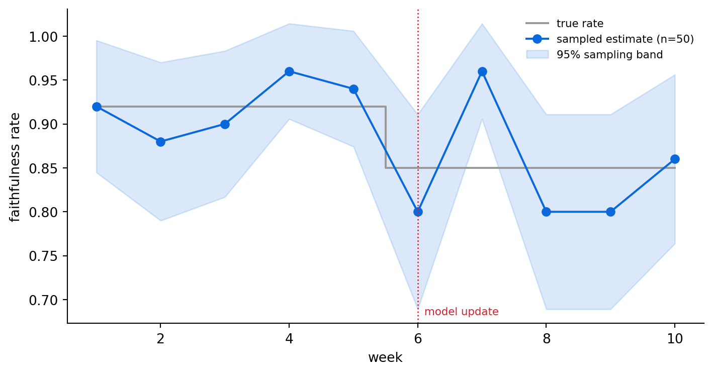
The drop is real from week six, but the sampled line does not announce it: for the first week or two after the update the estimate sits inside the band it occupied before, because a seven-point fall is small next to the wobble of a fifty-call sample. Only once several post-update weeks accumulate does the decline clearly separate from chance. This lag is the reason sample size is a monitoring decision as well as a cost one: a larger weekly sample tightens the band and shortens the delay, a smaller one saves money and lengthens it, and where you set the rate is a deliberate trade between detection speed and judge cost.
24.4 Detecting drift before users do
The inputs themselves change over time, and a model tuned for last quarter’s questions can quietly underperform on this quarter’s. You can catch this without any labels by watching the distribution of inputs. Embed a reference batch from when the system was known to be healthy, and compare new traffic against it. If new inputs sit far from the reference distribution, something has shifted.
from gaba.embed import embed_texts
from gaba.data import load_tickets

tickets = load_tickets()["text"].tolist()
reference = tickets[:18]               # a healthy baseline
new_similar = tickets[18:28]           # later traffic, same kind of tickets

# A reference centroid: the average direction of healthy inputs.
ref_vectors = embed_texts(reference)
centroid = ref_vectors.mean(axis=0)
centroid /= np.linalg.norm(centroid)

def drift_score(batch: list[str]) -> float:
    """Mean cosine distance of a batch from the reference centroid."""
    vectors = embed_texts(batch)
    return float(np.mean([1 - (v @ centroid) / np.linalg.norm(v) for v in vectors]))

print(f"drift of similar new traffic: {drift_score(new_similar):.3f}")
drift of similar new traffic: 0.336This score is the baseline drift, the measure of what normal variation looks like. Now compare a batch from a genuinely different distribution, standing in for the day your support inbox fills with a new kind of issue.
from datasets import load_dataset

other_domain = [r[:200] for r in
                load_dataset("stanfordnlp/imdb")["train"].shuffle(seed=0).select(range(10))["text"]]
print(f"drift of off-distribution traffic: {drift_score(other_domain):.3f}")
drift of off-distribution traffic: 0.506The off-distribution batch has a clearly higher drift than the similar one. In production you set a threshold from the normal variation and alert when new traffic crosses it, which tells you the inputs have shifted before anyone files a complaint, while you still have time to re-evaluate and adapt.
This clean separation is also where the simple metric can mislead. Because real drift rarely arrives as a clean swap of the whole batch, the realistic case is a fraction of new traffic that has shifted, a new issue type appearing alongside business as usual. Consider what the centroid does with a batch that is only half shifted.
half_shifted = list(new_similar[:5]) + other_domain[:5]
print(f"half-shifted batch drift: {drift_score(half_shifted):.3f}")
half-shifted batch drift: 0.435Half is one point on a curve. Sweeping the contaminated fraction from none to all and mixing in-distribution and off-distribution texts in each proportion, we draw the whole relationship between how much traffic has shifted and what the centroid metric reports.
fractions = [0.0, 0.25, 0.50, 0.75, 1.0]
pool_in, pool_out = list(new_similar), list(other_domain)
n_batch = 10
sweep_scores = []
rng = np.random.default_rng(0)
for frac in fractions:
    n_out = int(round(frac * n_batch))
    batch = ([pool_out[i % len(pool_out)] for i in range(n_out)]
             + [pool_in[i % len(pool_in)] for i in range(n_batch - n_out)])
    sweep_scores.append(drift_score(batch))

threshold = sweep_scores[-1] - 0.02   # an alert calibrated just under the full shift

fig, ax = plt.subplots(figsize=(6.5, 4))
ax.plot([f * 100 for f in fractions], sweep_scores, marker="o",
        color="#0969da", linewidth=2)
ax.axhline(threshold, color="#cf222e", linestyle="--", linewidth=1)
ax.text(2, threshold + 0.004, "alert threshold", fontsize=8, color="#cf222e")
missed = [f * 100 for f, s in zip(fractions, sweep_scores) if s < threshold]
if missed:
    ax.axvspan(0, max(missed), color="#bf8700", alpha=0.12)
ax.set_xlabel("off-distribution fraction of the batch (%)")
ax.set_ylabel("drift score (mean cosine distance)")
ax.spines[["top", "right"]].set_visible(False)
plt.tight_layout(); plt.show()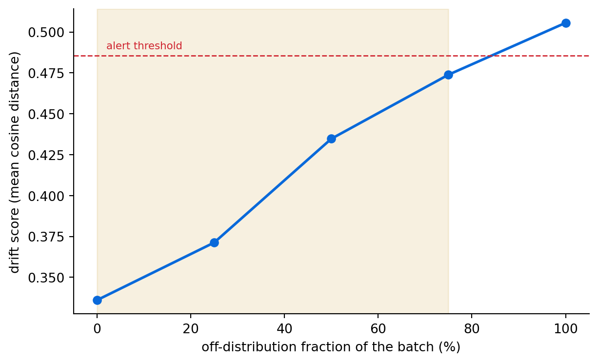
The curve rises with contamination, but it rises smoothly, which is the problem for any single threshold: set the alert just under the catastrophic full-shift score and the shaded band on the left is the whole range of partial shifts that pass underneath it, undetected, even though a quarter or half of the traffic has already turned over. The missed range follows from the metric’s design, which averages the shifted fraction against the calm one, so a finer measurement would not remove it. Lowering the threshold to catch the partial shifts trades the miss for false alarms on normal variation, which is the dilemma a mean-based detector cannot resolve and a distribution-level test can.
The three scores side by side make the dilution visible.
batch_names = ["similar\n(in-distribution)", "half-shifted", "different\n(off-distribution)"]
batch_scores = [drift_score(new_similar), drift_score(half_shifted),
                drift_score(other_domain)]

fig, ax = plt.subplots(figsize=(5.5, 3.5))
bars = ax.bar(batch_names, batch_scores,
              color=["#0969da", "#8250df", "#cf222e"], width=0.55)
ax.bar_label(bars, fmt="%.3f", padding=3)
ax.set_ylabel("drift score (mean cosine distance)")
ax.spines[["top", "right"]].set_visible(False)
plt.tight_layout()
plt.show()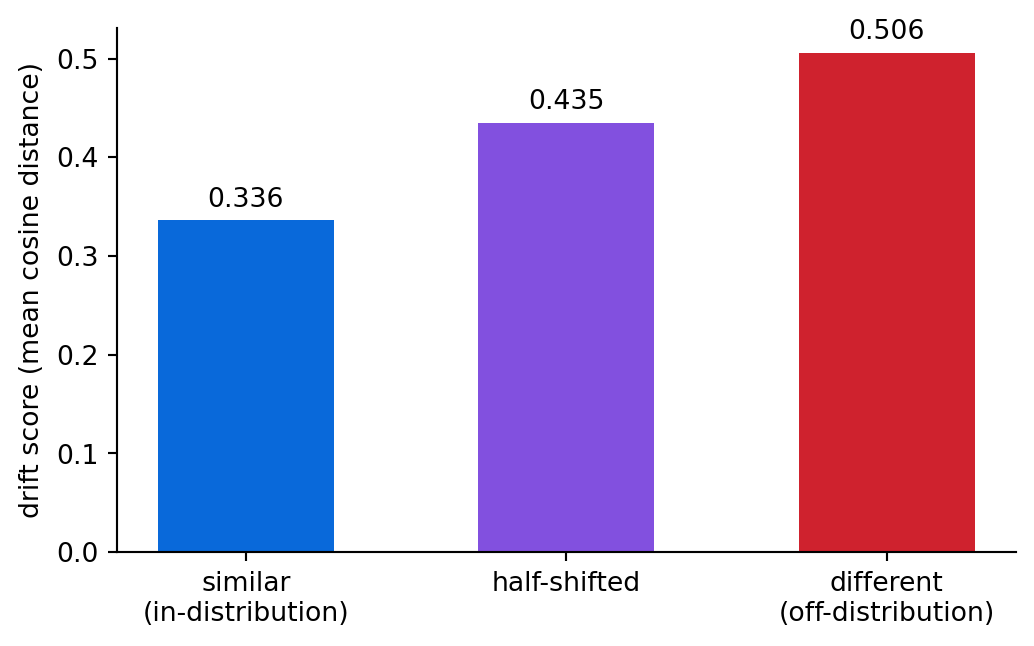
The score falls roughly midway between the baseline and the fully shifted batch, which is exactly what averaging predicts: the batch is half calm and half shifted, so its mean distance settles near the average of the two regimes. Because the score settles there, a threshold calibrated near the full-shift score, the obvious catastrophe, does not flag this batch even though half the traffic has changed, which makes the averaging weakness concrete: a mean-based detector dilutes exactly the partial shift we most want to catch early. The metric is deliberately simple, the mean cosine distance (one minus the cosine similarity of two vectors, so larger means more different) to a reference centroid, and that simplicity is also its blind spot. Stronger two-sample tests (which compare two whole distributions for any difference), such as maximum mean discrepancy (a single number for how far apart two whole distributions sit) or a per-dimension comparison, look at the whole distribution, whereas the centroid summarizes only its center, and so catch what a centroid cannot. Even so, the simple version still serves as a first alarm, because it needs no labels, which makes it the cheapest early-warning system you can run, as long as you remember what it cannot see.
WarningDon’t outsource this
Setting the alert threshold on drift_score is not a number an assistant should pick for you. The centroid metric averages a shifted fraction together with the calm majority, so a threshold tuned to catch the full-shift case is mathematically guaranteed to miss some partial shifts, and only you can decide how much of this blind spot your business can tolerate against the cost of false alarms. This trade belongs to the person who will answer the alerts, and no demo run can make it for them.
To see the blind spot directly, move the fraction of shifted traffic and the alert threshold, and observe where the alert fires and where it remains silent, noting that the expected score is the linear mixture of the two endpoints we just measured.
24.5 Kill switches and graceful failure
The last piece of observability is what happens when monitoring fires. A production system needs a way to fail safe: a circuit breaker that stops calling a provider that is down (since a naive client would retry forever), a kill switch that can disable an agent’s risky tools without a redeploy, and a fallback to a simpler model or cached answer when the primary errors. Observability tells you something is wrong; these mechanisms keep “wrong” from becoming “harmful” while you fix it.
24.6 Evaluation: does drift detection catch a shift?
The drift detector is itself a system, and we check it the same way: does it flag a shifted batch and not flag a normal one?
Metric: the drift score, which should be clearly higher for off-distribution input than for in-distribution input.
Test set: a batch of similar new traffic and a batch from a different distribution.
Baseline: the normal drift of in-distribution traffic, which sets the alert threshold.
import pandas as pd
pd.DataFrame({
    "batch": ["similar (in-distribution)", "different (off-distribution)"],
    "drift score": [round(drift_score(new_similar), 3), round(drift_score(other_domain), 3)],
})| batch | drift score | |
|---|---|---|
| 0 | similar (in-distribution) | 0.336 |
| 1 | different (off-distribution) | 0.506 |
The gap between the two is the signal. A real deployment computes the in-distribution drift over many healthy batches to learn its normal range, sets the alert threshold above that range, and watches. One caveat deserves emphasis: drift detection tells you the inputs changed, while whether quality dropped remains a separate question. The two usually go together, but the alert, which carries no verdict on its own, is a prompt to re-evaluate with the labeled tools of Chapter 9.
ImportantCompliance: traces are personal data
A trace captures the full prompt, and the full prompt contains whatever the customer wrote: names, account details, complaints, sometimes payment information. The trace store is therefore a store of personal data, and the retention, access, and residency rules of Appendix D apply to it just as they apply to the production database. Decide who can read traces, how long they are retained, and whether customer text needs masking before it is stored in a third-party observability platform.
TipCost: observability is cheap insurance
Tracing adds negligible cost, a small logging overhead per call. Production evaluation costs a judge call on a small sample, a few percent of traffic. Drift detection is embeddings you may already be computing. On self-hosted hardware the same arithmetic appears as capacity: tracing adds negligible latency per call, and a sampled judge consumes only a small fraction of the throughput that judging every call would take from the same machines. Against these small ongoing costs sits the cost of a silent failure running for a month, which is the expensive thing observability exists to prevent.
24.7 Exercises
24.7.1 Conceptual questions
The defining failure of production LLM systems is that they:
- Crash under load once traffic exceeds what testing covered
- Leak data through verbose error messages in production logs
- Grow more expensive each month as providers raise token prices
- Degrade silently, so no one notices until users complain
A trace of a model call should record:
- The inputs, output, and metadata: model, tokens, cost, and latency
- Only the final answer, since the inputs may contain user data
- The cost and latency alone, since the text is too large to store
- A hash of the conversation, so incidents can be matched without storing text
Why judge only a sampled few percent of production traffic?
- The judge model grows less accurate when it runs continuously
- A random sample gives a more representative picture of quality than full coverage
- Judging every call roughly doubles cost; a sample tracks quality cheaply
- Providers rate-limit judge calls to a fixed fraction of traffic
Drift detection works without labels by:
- Counting how often the model returns an error or an empty answer
- Comparing the distribution of new inputs against a healthy reference batch
- Asking a judge model to score a small sample of recent answers
- Re-running the launch evaluation set each week and watching the accuracy trend
A drift alert tells you:
- The inputs changed; the alert prompts a re-evaluation and carries no verdict on quality
- Answer quality has dropped by an amount proportional to the rise in the score
- The provider has silently updated the model behind the API
- The embedding model is stale and needs to be replaced with a newer one
In the chapter’s demo, the half-shifted batch scored 0.435, roughly midway between the 0.336 baseline and the 0.506 full shift, so a threshold set near the full-shift score would miss it. Why does the score land there?
- Half a batch is too small a sample for mean cosine distance to register the shift
- The off-distribution texts were truncated to 200 characters, weakening their signal
- The alert threshold was calibrated on the full shift, so the metric rescaled around it
- The centroid mean averages the calm half with the shifted half, landing at the mixture average
Which approach would catch the partial shift that the centroid metric dilutes?
- Lowering the alert threshold until even small score increases trigger an alert
- A two-sample test such as maximum mean discrepancy, comparing whole distributions
- Embedding both batches with a larger, more accurate embedding model
- Averaging the drift scores over a longer window to smooth out batch noise
In evaluating the drift detector itself, what plays the role of the baseline?
- The off-distribution batch, which sets the score the detector must reach
- Zero drift, since identical batches should always produce a score of zero
- The normal drift of in-distribution traffic, which sets the alert threshold
- The faithfulness rate the judge model assigns to the same batches of traffic
24.7.2 Build lab
Compute the drift score over five separate in-distribution batches to estimate the normal range, then set an alert threshold (for example, the mean plus two standard deviations). Run the off-distribution batch and confirm it crosses the threshold while the in-distribution batches do not. Report your threshold and whether it cleanly separates the two.
24.7.3 Evaluate lab
This one is yours to design. Build a small production-evaluation loop: take ten answers from any earlier chapter’s system, judge them with the Chapter 9 judge, and record the faithfulness rate. Then imagine a model change degraded three of them, recompute, and report how large a sample you would need to detect that drop reliably. Decide what sampling rate you would run in production.
NoteWhere we go next
We can build capabilities, make them safe, and watch them in production. The last chapter assembles it: Chapter 25 wraps the accumulated retrieval-and-agent system in a small web service with a chat interface, the eval harness and observability built in, so a colleague can finally use what we built.