from dotenv import load_dotenv
load_dotenv()

import networkx as nx
import matplotlib.pyplot as plt21 Knowledge graphs from text
Turning documents into a map of entities and relationships
Retrieval-augmented generation treats a corpus as an unstructured collection of chunks: it finds the passages nearest a question and returns them. This works well for questions like “what does this document say about X”, but it does not represent how things relate to each other: which companies supply which, which executives sit on which boards, and which acquisition connects two clusters of companies. A knowledge graph captures these relationships, with entities as nodes and typed relationships as edges, turning unstructured text into a structured map that you can traverse. In this chapter, we build a knowledge graph from a corpus of fourteen business-news snippets. We extract typed relationships, reconcile entity names, assemble and query the graph, and measure the extraction against ground truth, the foundation for the multi-hop questions of the next chapter. This Part sits in the specialize stage of the Chapter 1 lifecycle, giving the system structured knowledge it can traverse.
NoteSetup for this chapter
Run in the gaba-core environment with an OPENROUTER_API_KEY. This chapter introduces gaba.graph and uses networkx, an in-memory graph library, so no database server is needed; for production scale, the same graph goes into a database like Neo4j, which we note at the end. The corpus is fourteen fictional business-news snippets (assets/data/kg/) about an invented ecosystem of companies, some familiar from Chapter 19. The fiction is deliberate: the model cannot know these relationships from training data, so every edge in the graph provably came from the text, and the corpus includes a gold graph (the relationships a careful human reader confirms, our ground truth) that makes extraction quality measurable.
21.1 Tools in this chapter
| Tool | Why we use it here | Alternatives | Trade-off |
|---|---|---|---|
| networkx | an in-memory graph library; enough to build and query a graph with no server | Kùzu (embedded); Neo4j or Memgraph (servers) | zero setup against not scaling to millions of nodes |
| Neo4j | the common graph database for persistence and scale, noted here for production | Memgraph, ArangoDB | scale and a query language against running a service |
The tooling-landscape appendix lists the current options for each.
21.2 Extracting relationships
The unit of a knowledge graph is the triple: a subject, a relation, and an object, “Northwind Systems, ACQUIRED, Orchard Software.” Extracting triples is a structured-output task in the sense of Chapter 3: we describe the structure we want and let the model fill it from the text. One design decision matters most, and it happens before any prompt is written: the relations come from a fixed, typed vocabulary.
from gaba.graph import Relation, load_documents

print("relation vocabulary:", ", ".join(Relation.__args__))

docs = load_documents()
print(f"\n{len(docs)} documents; the first:\n\n{docs[0]}")
relation vocabulary: ACQUIRED, PARTNERS_WITH, INVESTS_IN, COMPETES_WITH, SUPPLIES_TO, SUBSIDIARY_OF, CEO_OF, BOARD_MEMBER_OF, FOUNDED
14 documents; the first:
Northwind Systems, the Seattle cloud-analytics firm, completed its acquisition of Orchard Software in March 2024. Orchard's forecasting tools will be folded into Northwind's platform. Elena Brandt, chief executive of Northwind Systems, called the deal the company's largest to date. Orchard Software was founded by Jonas Kim, who will stay on as a vice president.A controlled vocabulary is what makes a graph queryable. If the extractor may improvise, the same fact will arrive as “supplies”, “sells to”, and “is a supplier of” across documents, and the query “find every supplier” will silently miss two of the three. The schema in gaba.graph enforces the vocabulary with a Literal type, so an out-of-vocabulary relation, which would otherwise enter the graph as a quiet inconsistency, surfaces as a validation error the structured-output machinery rejects and retries, Chapter 3’s loud-failure principle applied to graph building.
flowchart LR
    sent["'Northwind Systems completed its<br/>acquisition of Orchard Software...<br/>Elena Brandt, chief executive of<br/>Northwind Systems...'"] --> ext["LLM extraction<br/>(structured output)"]
    ext --> nw["Northwind<br/>Systems"]
    nw -- "ACQUIRED" --> orc["Orchard<br/>Software"]
    brandt["Elena Brandt"] -- "CEO_OF" --> nw
from gaba.graph import extract_triples

triples = extract_triples(docs[0])
for t in triples:
    print(f"  ({t.subject}) -[{t.relation}]-> ({t.object})")
(Northwind Systems) -[ACQUIRED]-> (Orchard Software)
(Elena Brandt) -[CEO_OF]-> (Northwind Systems)
(Orchard Software) -[FOUNDED]-> (Jonas Kim)One paragraph of prose became a handful of typed facts. The extraction captured what a chunk could not: the relation is named and typed, whereas in a chunk it stays buried in the wording. An acquisition, a chief executive, and a founder are now three differently labeled edges that can each be queried by type.
21.3 The same company under different names
Before assembling a graph from all fourteen documents, we walk into one trap deliberately. Document four refers to “Northwind” where the other documents say “Northwind Systems”, the way follow-up coverage always shortens names. Extract it and look at the subject:
raw = extract_triples(docs[3])
for t in raw:
    print(f"  ({t.subject}) -[{t.relation}]-> ({t.object})")
(Northwind) -[ACQUIRED]-> (Orchard)
(Northwind) -[PARTNERS_WITH]-> (Meridian Semiconductors)
(Meridian Semiconductors) -[SUPPLIES_TO]-> (Northwind)
(Meridian Semiconductors) -[COMPETES_WITH]-> (Bluepeak Robotics)Left alone, “Northwind” and “Northwind Systems” become two unconnected nodes, and every traversal through the company silently loses the edges attached to the wrong one. This is entity resolution, the most common failure in real knowledge-graph pipelines. The fix is a canonicalization step that maps known variants onto one name. gaba.graph.canonicalize applies an alias table; at scale the table comes from string similarity, shared identifiers, or an entity-resolution model, but the step itself is never optional.
from gaba.graph import canonicalize

for t in canonicalize(raw):
    print(f"  ({t.subject}) -[{t.relation}]-> ({t.object})")
(Northwind Systems) -[ACQUIRED]-> (Orchard Software)
(Northwind Systems) -[PARTNERS_WITH]-> (Meridian Semiconductors)
(Meridian Semiconductors) -[SUPPLIES_TO]-> (Northwind Systems)
(Meridian Semiconductors) -[COMPETES_WITH]-> (Bluepeak Robotics)21.4 Building the graph
Now the full pipeline: extract every document, canonicalize, and assemble the edges into a networkx directed graph, which gaba.graph.build_knowledge_graph provides. The function persists the extracted triples to a small JSON cache (assets/data/cache/kg_triples.json), writing it on the first build and loading it on every later one, so that re-running this chapter, and Chapter 22 in its separate kernel, reuses exactly the same graph without a second round of extraction.
from gaba.graph import build_knowledge_graph

G = build_knowledge_graph()
print(f"nodes: {G.number_of_nodes()}, edges: {G.number_of_edges()}")
print("\nfirst ten entities:", sorted(G.nodes())[:10])
nodes: 32, edges: 37
first ten entities: ['Amara Diallo', 'Aurora Cell Works', 'Bluepeak Robotics', 'Cascadia Foods', 'Dev Sharma', 'Elena Brandt', 'Fernway Markets', 'Granite Bank', 'Helio Capital', 'Helios Energy Cooperative']Drawing the graph shows the structure the triples produced.
fig, ax = plt.subplots(figsize=(11, 7.5))
pos = nx.spring_layout(G, seed=7, k=0.6)
people = [n for n in G.nodes() if " " in n and not any(
    w in n for w in ["Systems", "Works", "Motors", "Foods", "Bank", "Group",
                     "Logistics", "Hotels", "Grid", "Capital", "Software",
                     "Dynamics", "Robotics", "Semiconductors", "Markets",
                     "Cooperative"])]
colors = ["#8250df" if n in people else "#0969da" for n in G.nodes()]
nx.draw_networkx(G, pos, ax=ax, node_color=colors, font_color="black",
                 node_size=900, font_size=7, edge_color="#b0b8c0", arrows=True,
                 verticalalignment="bottom")
nx.draw_networkx_edge_labels(G, pos, ax=ax, font_size=5.5,
                             edge_labels=nx.get_edge_attributes(G, "relation"))
ax.axis("off")
plt.tight_layout()
plt.show()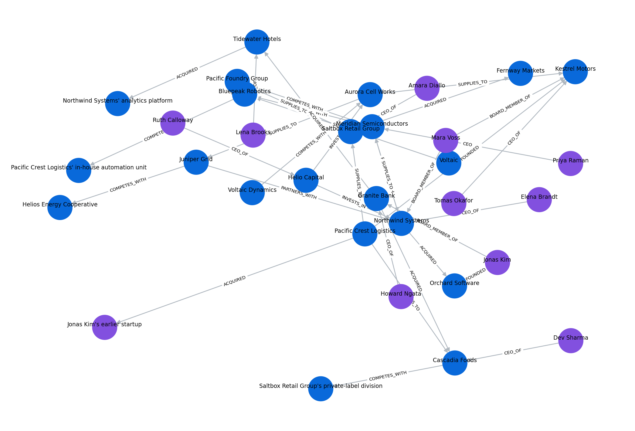
21.5 Querying the graph
Once the text is a graph, questions become graph operations, which are exact and explainable where similarity search is approximate. Three escalating examples follow. First, a node’s neighborhood, everything stated about one company:
TipWith an AI coding tool
Writing neighbors_out and neighbors_in as thin wrappers over G.successors and G.predecessors is exactly the boilerplate worth delegating, since the pattern is standard networkx and an assistant will get the syntax right on the first try. What deserves your own attention is the direction each wrapper queries, since a directed edge like ACQUIRED means something different read forward than read backward, and a wrapper that quietly swaps successors for predecessors would return a plausible-looking but wrong neighborhood with no error to catch it.
def neighbors_out(node):
    return [(G[node][n]["relation"], n) for n in G.successors(node)] if G.has_node(node) else []

def neighbors_in(node):
    return [(G[p][node]["relation"], p) for p in G.predecessors(node)] if G.has_node(node) else []

print("Northwind Systems, outgoing:")
for rel, obj in neighbors_out("Northwind Systems"):
    print(f"  -[{rel}]-> {obj}")
print("incoming:")
for rel, subj in neighbors_in("Northwind Systems"):
    print(f"  {subj} -[{rel}]->")
Northwind Systems, outgoing:
-[ACQUIRED]-> Orchard Software
-[PARTNERS_WITH]-> Meridian Semiconductors
incoming:
Elena Brandt -[CEO_OF]->
Meridian Semiconductors -[SUPPLIES_TO]->
Helio Capital -[INVESTS_IN]->
Mara Voss -[BOARD_MEMBER_OF]->
Juniper Grid -[PARTNERS_WITH]->Second, the benefit of the typed vocabulary: a query by relation type, across the whole graph at once. For example, every supply relationship in the corpus, regardless of which document stated it:
supply = [(u, v) for u, v, d in G.edges(data=True) if d["relation"] == "SUPPLIES_TO"]
for u, v in sorted(supply):
    print(f"  {u} -> {v}")
Aurora Cell Works -> Juniper Grid
Aurora Cell Works -> Kestrel Motors
Meridian Semiconductors -> Northwind Systems
Pacific Crest Logistics -> Cascadia Foods
Pacific Crest Logistics -> Saltbox Retail Group
Pacific Foundry Group -> Saltbox Retail Group
Voltaic -> Bluepeak RoboticsThird, a question no single document answers: which entities are the hubs this ecosystem depends on? Degree centrality, the number of edges touching each node, is the simplest graph analytic and already a useful one: a high-degree supplier is a concentration risk, and a high-degree person is the network’s connector.
import pandas as pd

degree = sorted(G.degree(), key=lambda kv: kv[1], reverse=True)[:6]
pd.DataFrame(degree, columns=["entity", "connections"])| entity | connections | |
|---|---|---|
| 0 | Northwind Systems | 7 |
| 1 | Meridian Semiconductors | 5 |
| 2 | Aurora Cell Works | 4 |
| 3 | Kestrel Motors | 4 |
| 4 | Saltbox Retail Group | 4 |
| 5 | Cascadia Foods | 4 |
Each row combines facts from multiple documents, the kind of question that takes an analyst an afternoon of reading and the graph a millisecond. The incoming-edges query, the by-type query, and the centrality table are all answers constructed from facts that were never stated together, which is the point of the graph.
Before we can trust this hub list, we compare it with the same top-6 computed from the gold graph, the edges a careful human reader found in the same fourteen documents.
from gaba.graph import load_gold

G_gold = nx.DiGraph()
for e in load_gold()["edges"]:
    G_gold.add_edge(e["s"], e["o"], relation=e["r"])

def top6(graph):
    ranked = sorted(graph.degree(), key=lambda kv: kv[1], reverse=True)[:6]
    return [f"{n} ({d})" for n, d in ranked]

pd.DataFrame({"extracted graph": top6(G), "gold graph": top6(G_gold)})| extracted graph | gold graph | |
|---|---|---|
| 0 | Northwind Systems (7) | Northwind Systems (8) |
| 1 | Meridian Semiconductors (5) | Meridian Semiconductors (5) |
| 2 | Aurora Cell Works (4) | Aurora Cell Works (4) |
| 3 | Kestrel Motors (4) | Kestrel Motors (4) |
| 4 | Saltbox Retail Group (4) | Saltbox Retail Group (4) |
| 5 | Cascadia Foods (4) | Cascadia Foods (4) |
Despite the edge-level errors we are about to measure, the two hub lists come out nearly identical: the same companies in the same order, with Northwind Systems on top either way and only its exact degree differing by the one edge extraction dropped. The noise did not propagate into the ranking here, and the reason is structural: the misses and extras are spread thinly across many nodes, so no single entity’s degree moves far enough to change its rank. This encouraging half of the result is corpus-specific, though. When extraction errors do concentrate, several mistyped edges all touching one company, that company’s centrality can move enough to indicate a concentration risk the documents never stated, which is why the rule still holds: compute the analytic both ways whenever you have gold, because extraction noise can propagate into every number built on the graph even when, this time, it did not.
21.6 Evaluation: did extraction capture the relationships?
Extraction is only useful if it captures what the text states, all of it and nothing else. Because the corpus includes a gold graph, the thirty-four edges a careful human reader finds in the fourteen documents, we can score both directions of failure.
Metric: recall (how many gold edges the extractor found) and precision (how many extracted edges are actually in the gold set). Recall catches what extraction missed; precision catches what it invented or mistyped.
Test set: the full gold graph in assets/data/kg/gold_graph.json.
Baseline: none; this establishes whether the graph is trustworthy at all.
from gaba.graph import load_gold

gold = {(e["s"], e["r"], e["o"]) for e in load_gold()["edges"]}
got = {(u, d["relation"], v) for u, v, d in G.edges(data=True)}

tp = gold & got
recall = len(tp) / len(gold)
precision = len(tp) / len(got)
print(f"gold edges: {len(gold)}  extracted: {len(got)}  matched: {len(tp)}")
print(f"recall: {recall:.2f}   precision: {precision:.2f}")

print("\nmissed (in gold, not extracted):")
for e in sorted(gold - got)[:4]:
    print("  ", e)
print("\nextra (extracted, not in gold):")
for e in sorted(got - gold)[:4]:
    print("  ", e)
gold edges: 34 extracted: 37 matched: 25
recall: 0.74 precision: 0.68
missed (in gold, not extracted):
('Bluepeak Robotics', 'COMPETES_WITH', 'Pacific Crest Logistics')
('Cascadia Foods', 'COMPETES_WITH', 'Saltbox Retail Group')
('Cascadia Foods', 'PARTNERS_WITH', 'Pacific Crest Logistics')
('Granite Bank', 'PARTNERS_WITH', 'Cascadia Foods')
extra (extracted, not in gold):
('Bluepeak Robotics', 'COMPETES_WITH', "Pacific Crest Logistics' in-house automation unit")
('Cascadia Foods', 'COMPETES_WITH', "Saltbox Retail Group's private-label division")
('Granite Bank', 'ACQUIRED', 'Cascadia Foods')
('Granite Bank', 'ACQUIRED', 'Tidewater Hotels')The same scoring, drawn as one picture: every edge either matched, was invented, or was missed.
import matplotlib.lines as mlines

matched, extra, missed = got & gold, got - gold, gold - got
overlay = nx.DiGraph()
for s, r, o in got | gold:
    overlay.add_edge(s, o)
pos_overlay = nx.spring_layout(overlay, seed=7, k=0.6)

fig, ax = plt.subplots(figsize=(11, 7.5))
nx.draw_networkx_nodes(overlay, pos_overlay, ax=ax, node_color="#f6f8fa",
                       edgecolors="#9a9a9a", node_size=700)
nx.draw_networkx_labels(overlay, pos_overlay, ax=ax, font_size=6.5,
                        verticalalignment="bottom")
for edge_set, color, style in [(matched, "#0969da", "solid"),
                               (extra, "#cf222e", "solid"),
                               (missed, "#9a9a9a", "dashed")]:
    nx.draw_networkx_edges(overlay, pos_overlay, ax=ax,
                           edgelist=[(s, o) for s, r, o in edge_set],
                           edge_color=color, style=style, width=1.6, arrows=True)
ax.legend(handles=[
    mlines.Line2D([], [], color="#0969da", label="matched (extracted, in gold)"),
    mlines.Line2D([], [], color="#cf222e", label="extra (extracted, not in gold)"),
    mlines.Line2D([], [], color="#9a9a9a", linestyle="--",
                  label="missed (in gold, not extracted)")],
    loc="lower left", fontsize=8, frameon=False)
ax.axis("off")
plt.tight_layout()
plt.show()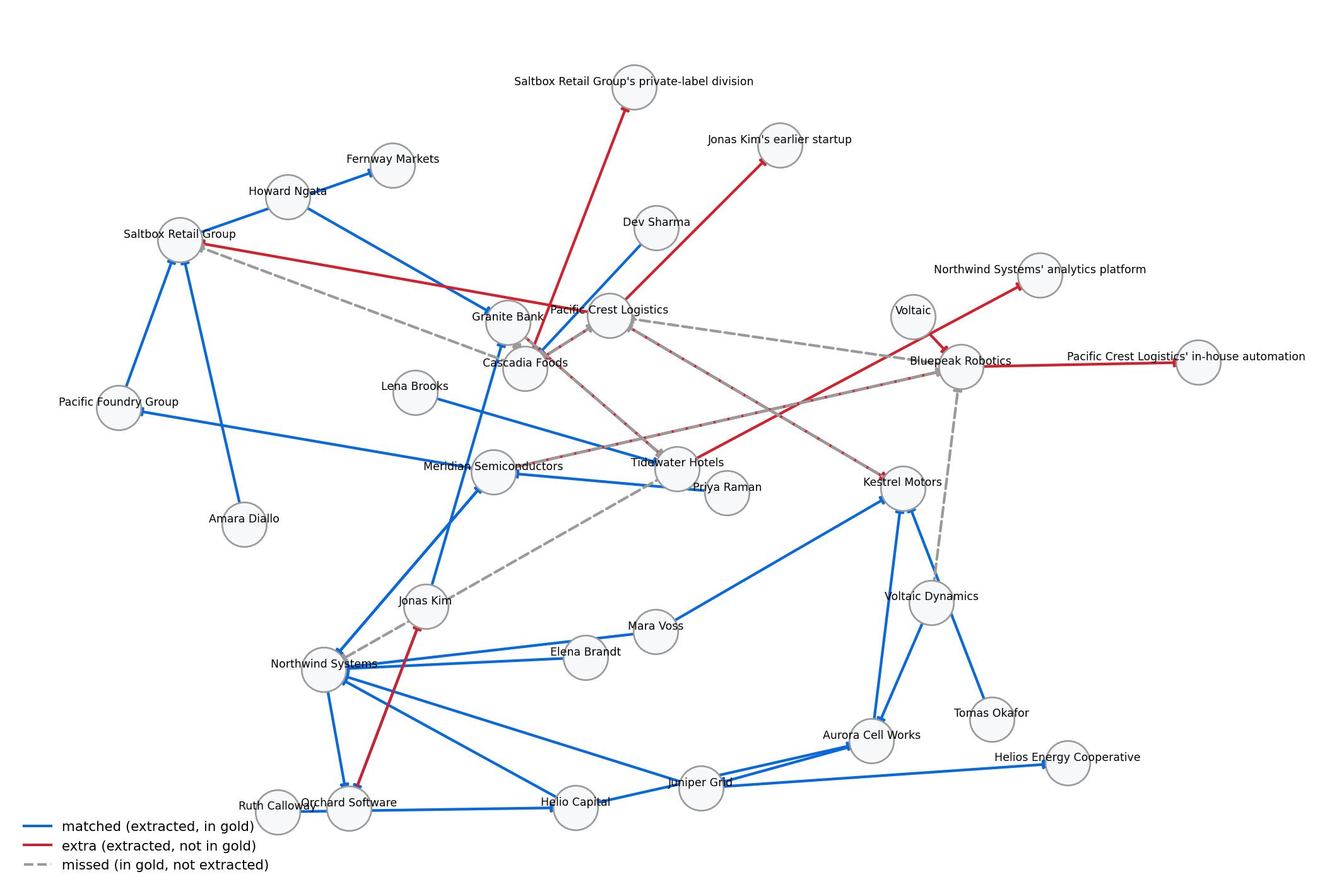
Read the two lists before trusting either number, because they diagnose the pipeline. The dominant pattern in our run is the possessive sub-entity: the text says a company competes with “Pacific Crest Logistics’ in-house automation unit”, and the extractor faithfully created that mouthful as its own node, although the relationship belongs to Pacific Crest Logistics itself, one error that costs a miss and an extra at once. The second pattern is the alias gap: “Voltaic” appears alongside “Voltaic Dynamics” because our alias table never anticipated that shortening, which is how alias tables grow in practice, one discovered variant at a time. Some extras are defensible paraphrases or true facts the gold list did not include, a reminder that the gold standard is itself a judgment. On real documents, where many relationships are only implied and names drift far more than our planted variants, both numbers fall, and this evaluation, run on a sample your team hand-labels, is how you decide whether the graph is complete enough to build on.
Patterns spotted by eye should also be counted. Because the extracted triples are cached and deterministic, every miss and extra can be hand-tagged with its failure type for an error analysis that tells you which fix to make first.
FAILURE_TYPES = {
    # extras: edges we extracted that gold does not contain
    ("Orchard Software", "FOUNDED", "Jonas Kim"): "paraphrase-or-direction",
    ("Voltaic", "SUPPLIES_TO", "Bluepeak Robotics"): "alias gap",
    ("Bluepeak Robotics", "COMPETES_WITH",
     "Pacific Crest Logistics' in-house automation unit"): "possessive sub-entity",
    ("Meridian Semiconductors", "COMPETES_WITH", "Bluepeak Robotics"): "mistype",
    ("Cascadia Foods", "COMPETES_WITH",
     "Saltbox Retail Group's private-label division"): "possessive sub-entity",
    ("Pacific Crest Logistics", "SUPPLIES_TO", "Kestrel Motors"): "paraphrase-or-direction",
    ("Pacific Crest Logistics", "FOUNDED", "Kestrel Motors"): "mistype",
    ("Pacific Crest Logistics", "SUPPLIES_TO", "Cascadia Foods"): "paraphrase-or-direction",
    ("Pacific Crest Logistics", "SUPPLIES_TO", "Saltbox Retail Group"): "true-extra",
    ("Tidewater Hotels", "ACQUIRED",
     "Northwind Systems' analytics platform"): "possessive sub-entity",
    ("Granite Bank", "INVESTS_IN", "Tidewater Hotels"): "paraphrase-or-direction",
    ("Granite Bank", "ACQUIRED", "Cascadia Foods"): "mistype",
    ("Granite Bank", "ACQUIRED", "Tidewater Hotels"): "mistype",
    ("Pacific Crest Logistics", "ACQUIRED",
     "Jonas Kim's earlier startup"): "possessive sub-entity",
    # misses: gold edges the extraction never produced
    ("Voltaic Dynamics", "SUPPLIES_TO", "Bluepeak Robotics"): "alias gap",
    ("Bluepeak Robotics", "COMPETES_WITH", "Pacific Crest Logistics"): "possessive sub-entity",
    ("Meridian Semiconductors", "SUPPLIES_TO", "Bluepeak Robotics"): "mistype",
    ("Cascadia Foods", "COMPETES_WITH", "Saltbox Retail Group"): "possessive sub-entity",
    ("Cascadia Foods", "PARTNERS_WITH", "Pacific Crest Logistics"): "paraphrase-or-direction",
    ("Kestrel Motors", "PARTNERS_WITH", "Pacific Crest Logistics"): "paraphrase-or-direction",
    ("Tidewater Hotels", "PARTNERS_WITH", "Northwind Systems"): "possessive sub-entity",
    ("Granite Bank", "PARTNERS_WITH", "Tidewater Hotels"): "paraphrase-or-direction",
    ("Granite Bank", "PARTNERS_WITH", "Cascadia Foods"): "mistype",
}

failures = pd.DataFrame([
    {"edge": f"{s} -[{r}]-> {o}"[:58],
     "failure": "extra" if (s, r, o) in got else "miss",
     "type": FAILURE_TYPES.get((s, r, o), "untagged")}
    for (s, r, o) in sorted(got ^ gold)])
pd.crosstab(failures["type"], failures["failure"])| failure | extra | miss |
|---|---|---|
| type | ||
| alias gap | 1 | 1 |
| mistype | 4 | 2 |
| paraphrase-or-direction | 2 | 3 |
| possessive sub-entity | 4 | 3 |
| true-extra | 1 | 0 |
The crosstab is the repair plan in priority order. Possessive sub-entities and the directional paraphrases dominate, and both are extraction-prompt problems: a rule that tells the extractor to attach every relationship to the named company even when the sentence mentions its unit or product, together with clearer direction examples, addresses most of the table. The alias gap is one line in a lookup table. The mistypes are the hard residue, the extractor reading a customer relationship as competition, and the true-extra row reflects a gap in the gold standard itself, since the extractor found a fact the labelers skipped. Counting failures by type turns “the extractor is mediocre” into “two prompt fixes and an alias entry recover most of the gap”, which is a statement a team can act on.
WarningDon’t outsource this
Hand-tagging each miss and extra with a failure type, possessive sub-entity, alias gap, mistype, is the step that turns a bare precision-and-recall score into a repair plan. An assistant could write the crosstab code in a moment, but deciding whether “Pacific Crest Logistics’ in-house automation unit” is a possessive sub-entity or a genuine new company requires you to read the source sentence and judge what the extractor should have done. That judgment is a reading task no model performed for us; it is what tells a team which prompt fix to make first, and the tooling does not supply it.
One more breakdown locates the weakest part of the vocabulary: recall by relation type.
relation_rows = []
for rel in sorted({r for _, r, _ in gold}):
    in_gold = sum(1 for _, r, _ in gold if r == rel)
    found = sum(1 for _, r, _ in tp if r == rel)
    relation_rows.append({"relation": rel, "gold edges": in_gold,
                          "matched": found, "recall": round(found / in_gold, 2)})
pd.DataFrame(relation_rows)| relation | gold edges | matched | recall | |
|---|---|---|---|---|
| 0 | ACQUIRED | 2 | 2 | 1.00 |
| 1 | BOARD_MEMBER_OF | 3 | 3 | 1.00 |
| 2 | CEO_OF | 8 | 8 | 1.00 |
| 3 | COMPETES_WITH | 5 | 3 | 0.60 |
| 4 | FOUNDED | 1 | 1 | 1.00 |
| 5 | INVESTS_IN | 2 | 2 | 1.00 |
| 6 | PARTNERS_WITH | 7 | 2 | 0.29 |
| 7 | SUPPLIES_TO | 6 | 4 | 0.67 |
The weakest relation in our run is PARTNERS_WITH, and the reason is visible in the anatomy table above: partnership is the vaguest relationship in the vocabulary, so the extractor keeps rendering it as something more specific, a supply deal, an investment, an acquisition. A recall-by-relation table like this is how you learn which parts of your schema the model can hear.
TipCost: one extraction call per document
Building the graph costs one structured-output call per document (or chunk of a long one), at a fraction of a cent each. This cost is paid once at indexing time, and then the graph is reused for every query after, just like embeddings. The graph queries themselves are free, since they run in memory and require no model call, which is part of the appeal. The expensive step is building the graph, whereas using it adds no further model cost.
The same is true on your own hardware: extraction is a one-time batch of model calls that will consume some throughput at indexing time, but traversals add no model latency at query time.
NoteFrom networkx to Neo4j
We used networkx because it needs no setup and our graph fits in memory. A real corpus produces a graph too large for that, and then you load the same triples, the ones our pipeline already persists as JSON in assets/data/cache/kg_triples.json, into a graph database such as Neo4j, which stores millions of nodes and replaces our Python calls with a query language (Cypher) for traversal. The supplier query above, in Cypher:
MATCH (s:Company)-[:SUPPLIES_TO]->(c:Company)
RETURN s.name, c.name
The extraction step remains the same, and only the store and the query syntax change. In production systems we often add a text-to-Cypher layer, a large language model translating analyst questions into queries against the discovered schema, which is the text-to-SQL pattern from Chapter 14 pointed at a graph.
21.7 Exercises
21.7.1 Conceptual questions
What does a knowledge graph capture that a flat pile of retrieved chunks does not?
- The exact wording of every sentence in the source documents
- A compressed summary of each document for faster retrieval
- The relationships between entities, stored as typed edges
- The embedding vector of each chunk, indexed for similarity search
The basic unit of a knowledge graph is:
- A triple: a subject, a relation, and an object
- A chunk: a fixed-size span of text from a source document
- A token: the smallest unit of text the model processes
- An embedding: a vector locating a text in semantic space
In this book’s terms, extracting triples from text is:
- A retrieval task, since the triples must be found in an index
- A clustering task, since related entities are grouped together
- A classification task, since each sentence is assigned a relation label
- A structured-output task with a schema the model fills from the text
The supplier query returned relationships that were stated in several different documents because:
- All supply relationships appeared together in one source document
- Separate documents became typed edges in one graph, queryable together
- The model recalled the connections from its training data
- The retriever ranked all the supplier chunks highest by similarity
A common difficulty when extracting a graph from real documents is:
- Graph libraries cannot hold more than a few thousand nodes in memory
- Models refuse to produce structured output from long, messy text
- Traversal queries become too slow to run without a GPU
- The same entity appears under varying names that must be reconciled
The chapter measures precision as well as recall against the gold graph. What does precision catch that recall cannot?
- Edges the extractor invented or mistyped, which recall alone would never see
- Edges the extractor missed, which precision weights by their importance
- Entity-name variants, which only show up as duplicated nodes
- Nothing extra; the two metrics always move together on extraction tasks
Where does the cost of a knowledge-graph pipeline concentrate?
- At query time, because every traversal of the graph requires its own model call
- In storage, because graph databases charge by the node and edge
- At indexing time: one extraction call per document, paid once
- Spread evenly, because each lookup re-extracts the relevant triples
When the corpus outgrows an in-memory networkx graph, what changes?
- The extraction prompt must be rewritten for the new database
- Only the store: the same triples load into a database like Neo4j
- The triples must be re-extracted in the query language of the new store
- Traversal is replaced by similarity search over node embeddings
21.7.2 Build lab
Extract a knowledge graph from one of the annual-report chunks (from the corpus used in Part II), which carry far messier text than the chapter’s clean snippets. Compare how clean the triples are, and note where entity names vary or relationships are missed. Report what you would add to the extraction prompt to handle real document text.
21.7.3 Evaluate lab
Run the chapter’s precision-and-recall evaluation on real text: take five paragraphs from one of the Part II annual reports, hand-label the relationships you can verify (your own small gold set), extract with the chapter’s pipeline, and report both numbers. Compare them to the clean-corpus scores and identify which failure grew more, the misses or the extras, and what you would change first.
NoteWhere we go next
The graph we can now query by hand becomes more useful still when a model can reason over it. In Chapter 22, we build Graph RAG, which answers a natural-language question by traversing the graph to gather connected facts, then handing them to a model. The model can then answer multi-hop questions that flat retrieval cannot.