flowchart TB
    hay["haystack: thousands of tokens of realistic filler text"] --> ctx["one assembled context"]
    needle["the needle: one planted fact<br/>('the vault code is 7414')<br/>inserted at depth d%"] --> ctx
    ctx --> q["question: what is the vault code?"]
    q --> verdict["found / missed,<br/>per (length, depth) cell"]
Appendix B — Appendix B: Benchmarking LLMs
The evaluation toolkit in Chapter 9 measures your system on your data. This appendix is about the other kind of measurement: benchmarking the models themselves, the standardized tests that tell you what a model can do before you build on it. These are useful for shortlisting models, and misleading if you mistake a leaderboard score for performance on your task.
B.1 What the standard benchmarks measure
Public benchmarks each probe one capability. A few worth knowing:
- Knowledge and reasoning (MMLU, Massive Multitask Language Understanding, and successors): multiple-choice questions across many subjects. The original MMLU is heavily saturated at the top (top models all score near the ceiling, so it no longer separates them); MMLU-Pro and GPQA (a graduate-level science set built to resist memorization) are where current models still separate.
- Coding (LiveCodeBench, SWE-bench): can the model write correct code or fix a real GitHub issue? The older HumanEval is saturated and no longer separates serious models. LiveCodeBench refreshes its problems over time to resist contamination, and SWE-bench in particular tracks agentic coding ability.
- Math (MATH and harder successors): multi-step reasoning, where reasoning models pull ahead. The long-time standard GSM8K is saturated, so a perfect score there is a given and carries no signal.
- Long context (needle-in-a-haystack): can the model find a fact buried in a very long input?
- Instruction following and chat (arena-style human preference): which model’s answers people prefer, head to head.
The caution is constant: although a high benchmark score is necessary, it is never sufficient. Models are sometimes trained on data that resembles the benchmarks, which is why the saturated ones above stopped being informative. A benchmark never looks exactly like your documents, your customers, or your task. Use benchmarks to shortlist, then run Chapter 9’s evaluation on your own data to decide.
Language models are not the only models with a leaderboard. The Massive Text Embedding Benchmark (MTEB) plays the same role for embedding models and rerankers. It scores them across retrieval, classification, and clustering tasks in many languages. This book runs on BGE-M3 (Chapter 6), and MTEB is where you would compare its successors when the time comes to upgrade. As before, shortlist from the leaderboard, then measure retrieval quality on your own corpus before switching, because re-embedding a corpus is not free (Appendix E).
B.2 A needle-in-a-haystack test you can run
The idea in one picture: a long stretch of realistic text, one planted fact, and a question that can only be answered by finding it.
The long-context test is easy to run yourself and is worth running because long-context behavior varies considerably between models. To perform the test, you hide a fact (the needle) at some depth in a long stretch of realistic filler text (the haystack) and then ask for it back. We run the full grid: three context lengths, roughly 2,000, 20,000, and 60,000 tokens of text drawn from the book’s annual-report corpus, crossed with three depths, the needle near the start, the middle, and the end.
from dotenv import load_dotenv
load_dotenv()
import pandas as pd
from gaba import DATA_DIR
from gaba.llm import call_llm
from gaba.rag import REPORTS

# Realistic filler: the report corpus itself, which looks like the documents
# a long-context model would be asked to read.
haystack_source = " ".join(
    (DATA_DIR / "filings" / filename).read_text() for filename in REPORTS.values()
)
secret = "The internal project codename is Bluefin."

# This markdown-heavy corpus runs a little over 5 characters per token, so
# these slice sizes land near the advertised token counts.
lengths = {"~2k tokens": 10_000, "~20k tokens": 100_000, "~60k tokens": 320_000}
depths = {"start": 0.05, "middle": 0.50, "end": 0.95}

rows = []
for length_label, chars in lengths.items():
    filler = haystack_source[:chars]
    for depth_label, depth in depths.items():
        pos = int(len(filler) * depth)
        context = filler[:pos] + " " + secret + " " + filler[pos:]
        reply = call_llm(f"{context}\n\nWhat is the internal project codename?",
                         system="Answer from the text.")
        rows.append({"length": length_label, "depth": depth_label,
                     "found": "bluefin" in reply.text.lower()})

grid = (pd.DataFrame(rows)
        .pivot(index="length", columns="depth", values="found")
        .reindex(index=list(lengths), columns=list(depths))
        .map(lambda found: "found" if found else "MISSED"))
grid| depth | start | middle | end |
|---|---|---|---|
| length | |||
| ~2k tokens | found | found | found |
| ~20k tokens | found | found | found |
| ~60k tokens | found | found | found |
import numpy as np
import matplotlib.pyplot as plt

mat = grid.replace({"found": 1, "MISSED": 0}).to_numpy(dtype=float)
fig, ax = plt.subplots(figsize=(5.5, 3.2))
ax.imshow(mat, cmap=plt.matplotlib.colors.ListedColormap(["#cf222e", "#2da44e"]),
          vmin=0, vmax=1, aspect="auto")
ax.set_xticks(range(len(grid.columns)), grid.columns)
ax.set_yticks(range(len(grid.index)), grid.index)
ax.set_xlabel("needle depth"); ax.set_ylabel("context length")
for r in range(mat.shape[0]):
    for c in range(mat.shape[1]):
        ax.text(c, r, "found" if mat[r, c] else "MISSED", ha="center",
                va="center", color="white", fontsize=10, fontweight="bold")
plt.tight_layout(); plt.show()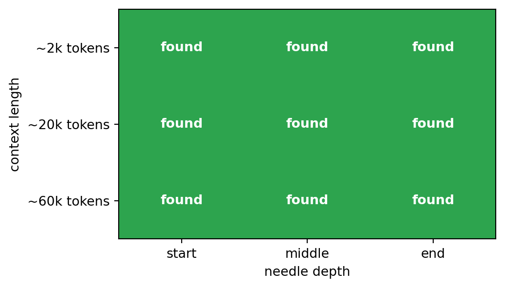
Read the grid for the pattern the cells draw, since the location of any failures carries more information than the overall verdict. A current frontier-tier model will likely fill every cell with “found”, sixty thousand tokens included; simple fact retrieval is the long-context task modern models have largely solved, and a clean grid here says so. A common mistake is to conclude from a clean sweep that the test is pointless. The grid is the method: any cell that reads “MISSED” tells you exactly which length-and-depth combination the model cannot be trusted with, and a clean sweep tells you that single-fact lookup is safe at these lengths for this model, nothing more. Where lost-in-the-middle still bites is reasoning over many facts spread through a long context (Chapter 10 measures a version of that), so a passed needle test does not clear a model for multi-fact synthesis. Rerun this grid with the model you are considering, at the lengths your documents reach, and with the cheap model swapped for the one you would deploy, before you rely on either to read long documents.
B.3 Benchmarking for your own use
The benchmark that matters most is the one you build: a held-out set of your real tasks with known answers, run against each candidate model. It is the only test that measures the thing you care about. Treat public benchmarks as a coarse filter to pick two or three candidates, then let your own evaluation, Precision@k for retrieval, accuracy for classification, LLM-as-judge for open answers, make the call. The recurring lesson of this book applies to model selection too: measure on your data, decide with a number.