17  Synthetic data, distillation, and the real-plus-synthetic mix

Generating training data that helps

Fine-tuning needs labeled examples, and the most common reason teams do not fine-tune is that they do not have enough. A large model can supply them: ask it to write labeled examples, or to label data you already have, and you get a training set for a fraction of the cost of human labeling. This is synthetic data, and when a big model’s output trains a smaller, cheaper one, it is called distillation. Asking whether synthetic data is good or bad in general leads nowhere; the useful question is when it helps, and this chapter answers it with one experiment: synthetic data helps most when real data is scarce, and the benefit fades as you accumulate real data. We will watch it help a lot, watch it stop helping, and draw the rule that follows: synthetic data is an amplifier for scarce real data, and you confirm its value by measuring against real data every time.

NoteSetup for this chapter

Run in the gaba-core environment with an OPENROUTER_API_KEY. We generate examples by API and train small classifiers on embeddings, on CPU, so no GPU is needed. We use a public emotion-classification dataset as the “real” data to test against. The dataset and the embedding model download from Hugging Face on a first run.

from dotenv import load_dotenv
load_dotenv()

import numpy as np
import pandas as pd
import matplotlib.pyplot as plt
from datasets import load_dataset
from sklearn.linear_model import LogisticRegression
from gaba.llm import call_llm, MODEL_DEFAULT, MODEL_LIGHT
from gaba.embed import embed_texts

17.1 Generating synthetic data

The mechanic is simple: ask a model to produce labeled examples. We choose a harder task than binary sentiment on purpose. Emotion classification has six classes, and the distinctions are subtle (love versus joy, fear versus surprise), so a handful of real examples per class genuinely limits a classifier. This is the setting where synthetic data has a gap to fill; on an easy task, a good embedding model already succeeds from a few examples, and there is nothing left to add. (The running example meets the same scarce-label setting when a new ticket category appears: five real examples of a brand-new complaint type is exactly this problem as it shows up at work.)

EMOTIONS = {0: "sadness", 1: "joy", 2: "love", 3: "anger", 4: "fear", 5: "surprise"}

def generate_examples(label: int, n: int) -> list[str]:
    emotion = EMOTIONS[label]
    out = []
    for i in range(n):
        # Temperature 1.0 and a "vary the situation" nudge: a synthetic set with
        # no variety teaches the classifier nothing.
        r = call_llm(f"Write one short first-person sentence, like a tweet, that "
                     f"clearly expresses {emotion}. Vary the situation. #{i}",
                     system="You write short, varied emotional social-media sentences.",
                     temperature=1.0)
        out.append(r.text.strip())
    return out

synth_texts, synth_labels = [], []
for label in EMOTIONS:
    synth_texts += generate_examples(label, 25)   # 25 per class
    synth_labels += [label] * 25

print(f"generated {len(synth_texts)} synthetic examples across {len(EMOTIONS)} emotions")
print("sadness:", synth_texts[0])
print("joy:    ", synth_texts[25])

generated 150 synthetic examples across 6 emotions
sadness: My favorite mug is chipped, and it feels like the last straw.
joy:     My heart is just bursting right now because I got the promotion! 🥳

In minutes and for pennies, we produced a labeled set for all six emotions. The examples are plausible, but they are not real: they reflect how the model writes a tweet, and the model’s manner of writing differs from how people actually write one. Whether that matters turns out to depend entirely on how much real data we already have.

17.2 When does synthetic data help? It depends on what you already have

To find out, we hold a real test set fixed and vary how much real training data we give the classifier, from very scarce (five examples per class) to comfortable (forty per class). At each level, we compare training on the real data alone against training on the real data plus all of our synthetic examples. We average each comparison over three random draws of the real subset to make sure one lucky or unlucky draw does not determine the result. We use embeddings as features (Chapter 13) because a semantic representation will place a synthetic sentence near the real sentences it resembles, even when the exact words are different.

emotion = load_dataset("dair-ai/emotion")
by_class = {k: [] for k in EMOTIONS}
for row in emotion["train"]:
    by_class[row["label"]].append(row["text"])
test_texts = emotion["test"]["text"][:500]
test_labels = np.array(emotion["test"]["label"][:500])

# A real pool to draw scarce subsets from, embedded once alongside the rest.
pool_texts, pool_labels = [], []
for k in EMOTIONS:
    pool_texts += by_class[k][:40]
    pool_labels += [k] * 40
pool_labels = np.array(pool_labels)

vectors = embed_texts(pool_texts + synth_texts + list(test_texts))
n_pool, n_synth = len(pool_texts), len(synth_texts)
E_pool, E_synth, E_test = vectors[:n_pool], vectors[n_pool:n_pool + n_synth], vectors[n_pool + n_synth:]

def score(X, y) -> float:
    clf = LogisticRegression(max_iter=1000, class_weight="balanced").fit(X, y)
    return (clf.predict(E_test) == test_labels).mean()

rows = []
runs = {"real only": [], "real + synthetic": []}  # per-seed scores, kept for the plot's bands
for k in [5, 10, 20, 40]:
    real_only_runs, real_plus_runs = [], []
    for seed in range(3):  # three random draws of the real subset, averaged
        rng = np.random.RandomState(seed)
        idx = np.concatenate([rng.choice(np.where(pool_labels == c)[0], size=k, replace=False)
                              for c in EMOTIONS])
        X_real, y_real = E_pool[idx], pool_labels[idx]
        real_only_runs.append(score(X_real, y_real))
        real_plus_runs.append(score(np.vstack([X_real, E_synth]), list(y_real) + synth_labels))
    runs["real only"].append(real_only_runs)
    runs["real + synthetic"].append(real_plus_runs)
    real_only = float(np.mean(real_only_runs))
    real_plus = float(np.mean(real_plus_runs))
    rows.append({"real per class": k, "real only": round(real_only, 3),
                 "real + synthetic": round(real_plus, 3),
                 "gain": round(real_plus - real_only, 3)})

sweep = pd.DataFrame(rows)
sweep

	real per class	real only	real + synthetic	gain
0	5	0.410	0.496	0.086
1	10	0.440	0.499	0.059
2	20	0.506	0.521	0.015
3	40	0.512	0.532	0.020

Read the gain column top to bottom; each row is the mean of three random draws of the real subset. When real data is scarcest, five examples per class, adding synthetic data lifts accuracy by well over ten points. As we add real data the gain shrinks, and by forty examples per class it is small. The picture is clearer still as a plot.

fig, ax = plt.subplots(figsize=(7, 4))
ks = sweep["real per class"]
for name, color in [("real only", "#57606a"), ("real + synthetic", "#0969da")]:
    per_seed = np.array(runs[name])           # one row per size, one column per seed
    label = name if name == "real only" else f"real + {n_synth} synthetic"
    ax.plot(ks, per_seed.mean(axis=1), marker="o", color=color, label=label)
    ax.fill_between(ks, per_seed.min(axis=1), per_seed.max(axis=1),
                    color=color, alpha=0.15, linewidth=0)
ax.set_xlabel("real examples per class")
ax.set_ylabel("accuracy on real test")
ax.set_title("Synthetic data helps most when real data is scarce")
ax.legend(frameon=False)
ax.spines[["top", "right"]].set_visible(False)
plt.tight_layout(); plt.show()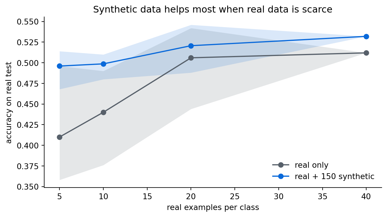

Figure 17.1: Accuracy on the real test set as real training data grows, averaged over three random draws of the real subset; the shaded bands span the minimum and maximum of the three runs (n=3). The two lines start far apart and converge, and the bands barely overlap at the scarce end, so the gap is not an artifact of one lucky draw.

The two lines start far apart and converge. This gap is the value of synthetic data, and it closes as real data grows. The same pattern recurs widely in published work on model-generated training data, and our sweep reproduces it, large gains that shrink toward nothing once the real set is large enough (often a few hundred to a thousand examples, depending on the task). Synthetic data is most valuable exactly when you have the least real data, which is also when you most want it.

17.3 Why it works, and where it stops

The mechanism is a trade. Each synthetic example is worth less than a real one, because it carries the model’s habits, whereas a real example carries the world’s. But synthetic examples are nearly free, so you can make a lot of them. When you are starved for data, an abundance of cheap, slightly-off examples beats a handful of real ones, because the classifier needs coverage of each class more than it needs perfect fidelity. Once you have enough real data, the trade reverses: real quality wins, and the slightly-off synthetic examples stop helping and eventually begin to reduce accuracy, which is the small negative drift you would see if we pushed the real set higher.

The “slightly off” is literal enough to see in the embedding space. We project the real pool and the synthetic set onto the same two principal components and look at where each cloud sits.

from sklearn.decomposition import PCA

coords = PCA(n_components=2, random_state=0).fit_transform(np.vstack([E_pool, E_synth]))
real_xy, synth_xy = coords[:n_pool], coords[n_pool:]

fig, ax = plt.subplots(figsize=(7, 5))
ax.scatter(real_xy[:, 0], real_xy[:, 1], facecolors="none", edgecolors="#9a9a9a",
           s=28, linewidths=0.8, label="real")
ax.scatter(synth_xy[:, 0], synth_xy[:, 1], color="#0969da", s=18, alpha=0.7,
           label="synthetic")
ax.set_xlabel("first principal component")
ax.set_ylabel("second principal component")
ax.legend(frameon=False)
ax.spines[["top", "right"]].set_visible(False)
plt.tight_layout(); plt.show()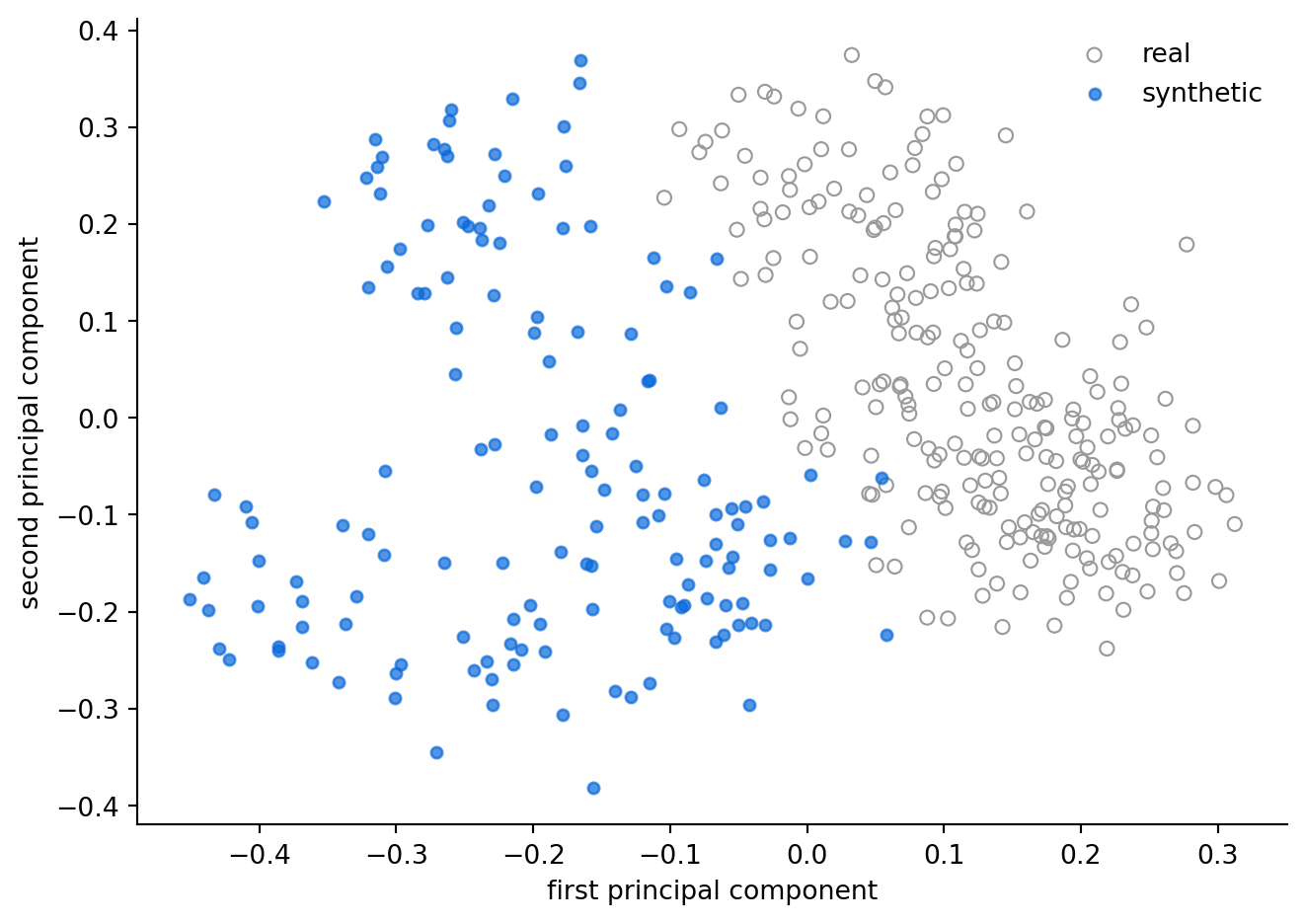

Figure 17.2: The real pool and the synthetic set projected onto the same two principal components. The synthetic cloud is tighter than the real one and sits slightly offset from it: a narrowed echo of the real distribution.

The synthetic cloud covers less of the space than the real one, and its mass sits slightly to one side of the real cloud’s, a small distribution shift: the model writes a narrower, more uniform version of each emotion than people do. Train on the tight cloud alone and the classifier learns the model’s narrowed version of each emotion, since that narrowed version is the only distribution it ever sees.

This same trade underlies model collapse. A synthetic example is a slightly distorted echo of the real distribution. If you train on synthetic data alone, and then train the next model on the output of the first, the distortion compounds across generations until quality drifts away from reality. The defense is the rule the experiment already points to: never train on a purely synthetic set across generations, always keep real data in the mix, and always test against real data you trust.

17.4 Distillation: labeling the real data we already have

There is a second way to use a large model that sidesteps this quality penalty almost entirely, and in production it is the more common approach. Where the previous section invented text from nothing, here you take real text that you already have but have not labeled, and have the large model label it. A small, cheap model then trains on those labels. This is called distillation. The key difference here is that the text stays real, and only the labels are synthetic. As a result, the distribution the small model learns is the true distribution. The economics are the payoff Chapter 15 promised: the expensive model labels the data once, and the small model that learns from it runs for almost nothing forever, inheriting much of the big model’s skill on that one task. The same discipline still applies: the small model is only as good as the labels it learns from, so you check those labels against a sample of human-verified ones before you trust the result.

The experiment is cheap enough to run, so we take 200 real sentences our classifier has never seen, have the big model label them, and train the same classifier twice, once on the model’s labels and once on the dataset’s gold labels.

LABEL_WORDS = ", ".join(EMOTIONS.values())

def teacher_label(text: str, model: str = MODEL_DEFAULT) -> int:
    r = call_llm(f"Classify the emotion of this sentence as exactly one of: "
                 f"{LABEL_WORDS}.\nSentence: {text}",
                 system="You classify emotions. Answer with one emotion word only.",
                 model=model)
    word = r.text.strip().lower()
    for label, name in EMOTIONS.items():
        if name in word:
            return label
    return -1  # a reply naming no emotion becomes a label that is always wrong

distill_texts = emotion["train"]["text"][10000:10200]   # real text, unseen above
distill_gold = np.array(emotion["train"]["label"][10000:10200])
teacher_labels = np.array([teacher_label(t) for t in distill_texts])

E_distill = embed_texts(list(distill_texts))
print(f"teacher agrees with gold labels: {(teacher_labels == distill_gold).mean():.0%}")
print(f"trained on gold labels:    accuracy {score(E_distill, distill_gold):.3f}")
print(f"trained on teacher labels: accuracy {score(E_distill, teacher_labels):.3f}")

teacher agrees with gold labels: 55%
trained on gold labels:    accuracy 0.570
trained on teacher labels: accuracy 0.500

Agreement is one number; where the teacher disagrees is a diagnosis. A confusion matrix of gold labels against teacher labels shows which emotions the teacher actually mixes up.

names = list(EMOTIONS.values())
conf = np.zeros((6, 6), dtype=int)
for g, t in zip(distill_gold, teacher_labels):
    if t >= 0:                       # drop the rare reply that named no emotion
        conf[g, t] += 1

fig, ax = plt.subplots(figsize=(6, 5))
ax.imshow(conf, cmap="Blues")
ax.set_xticks(range(6), names, rotation=45, ha="right")
ax.set_yticks(range(6), names)
ax.set_xlabel("teacher label")
ax.set_ylabel("gold label")
for i in range(6):
    for j in range(6):
        if conf[i, j]:
            ax.text(j, i, conf[i, j], ha="center", va="center", fontsize=9,
                    color="white" if conf[i, j] > conf.max() / 2 else "#1f2328")
plt.tight_layout(); plt.show()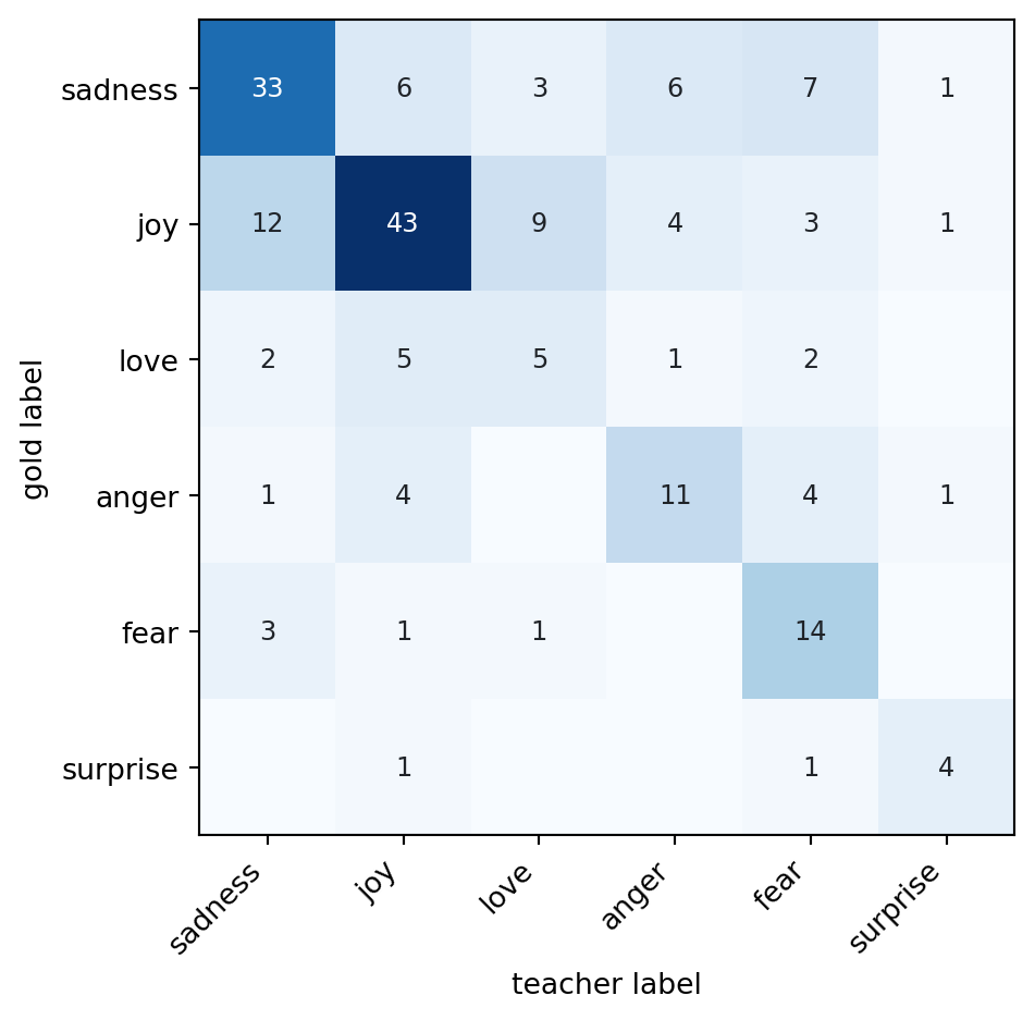

Figure 17.3: Teacher labels against gold labels for the 200 distillation sentences. The diagonal is agreement, and in our run the off-diagonal counts pile up between the adjacent emotions, love read as joy and surprise confused with fear, the same subtle distinctions that made this task worth choosing.

TipWith an AI coding tool

The confusion-matrix heatmap above, the six-by-six grid, the annotated counts, the color scale, is standard matplotlib boilerplate an assistant will draft correctly from a one-line request, although all it delivers is a grid of numbers on screen. Reading which off-diagonal cells actually carry weight, and noticing that they cluster between love and joy or between fear and surprise where random errors would scatter evenly, is the diagnosis only you can make once the plot is drawn.

The disagreements concentrate in a few adjacent pairs, which matters because a student inherits the teacher’s specific confusions. A common mistake is to picture the teacher’s errors as a uniform rate spread across the grid; because the errors concentrate, a pair the teacher cannot separate is a pair the student will never learn to separate, no matter how many labels we buy.

The gap between the two accuracies is the cost of the teacher’s labeling errors, and the agreement number is the early warning that predicts it: a teacher that disagrees with gold labels often will pass those disagreements straight into the student. This is distillation in miniature, with real text, model labels, a cheap student, and most of the quality. On a production task, you would label thousands of examples where we labeled 200, and you would verify a human-checked sample of the labels first, exactly as the previous paragraph prescribed.

The early warning shows its value when the teacher gets worse. We relabel the same 200 sentences with the cheaper MODEL_LIGHT and place the two teachers side by side.

from concurrent.futures import ThreadPoolExecutor

with ThreadPoolExecutor(max_workers=8) as ex:
    light_labels = np.array(list(ex.map(
        lambda t: teacher_label(t, model=MODEL_LIGHT), distill_texts)))

pd.DataFrame([
    {"teacher": MODEL_DEFAULT,
     "agreement with gold": f"{(teacher_labels == distill_gold).mean():.0%}",
     "student accuracy": round(score(E_distill, teacher_labels), 3)},
    {"teacher": MODEL_LIGHT,
     "agreement with gold": f"{(light_labels == distill_gold).mean():.0%}",
     "student accuracy": round(score(E_distill, light_labels), 3)},
])

	teacher	agreement with gold	student accuracy
0	google/gemini-2.5-flash-lite	55%	0.50
1	meta-llama/llama-3.1-8b-instruct	43%	0.47

In our run the two columns move together: the weaker teacher agrees with the gold labels less often, and its student scores lower. This is exactly what makes agreement useful as an early warning: it can be measured on a small human-verified sample before any student is trained, and it predicts how much quality the student is about to inherit.

One legal caveat before you distill from a commercial model: most providers’ terms of service restrict using their outputs to train models that compete with theirs, and some forbid it outright. Check the terms of the teacher you plan to use, or distill from an open-weight teacher whose license permits it. Appendix D’s compliance checklist is the place to record that check.

17.5 Evaluation: test on real, always

The evaluation in this chapter is the sweep itself, and its design carries the one rule that matters about evaluating synthetic data.

Metric: accuracy on a held-out set of real examples.
Test set: real, held-out sentences.
Baseline: the model trained on the real data alone, which is what synthetic data has to improve on to be worth anything.

The non-negotiable is that the test set is real. A model trained on synthetic data and evaluated on synthetic data can look excellent and be useless, because it is graded on the same distorted distribution it learned. The moment you test against real data, the real result appears: a gain when data is scarce, nothing when it is plentiful. Every claim that synthetic data “works” should be met with the question of what it was tested against, because unless the answer is real, held-out data, the claim is empty.

TipCost: synthetic data is cheap, the wrong call is expensive

Generating this synthetic set cost pennies, against hours of human labeling, which is exactly why the technique is so tempting. On hardware you own the dollars in the same arithmetic become time: generating the set takes minutes of GPU throughput, and the sweep is still what tells you whether those minutes were well spent. Because the generation cost is trivial either way, the real risk is spending real effort on synthetic data in a regime where it does not help, or worse, letting it quietly degrade a model that already had enough real data. The cheap step is generation; the necessary step is the sweep above, which measures whether, for your amount of real data, synthetic data still helps.

WarningDon’t outsource this

An assistant will generate all the synthetic data you ask for, instantly and convincingly. It will not tell you that you already have enough real data for it not to matter, or that your test set is also synthetic and therefore lying to you. The judgment of when synthetic data helps, and the discipline of always testing on real data, are yours.

17.6 Choosing your customization stack

Part VI decided when to fine-tune, trained a LoRA, and mixed synthetic data with real. The tools split into training, fitting the model in memory, and generating data.

Capability	Open-weight	Hosted	Choose by
Fine-tuning	Hugging Face PEFT and TRL, Axolotl, Unsloth	OpenAI, Together, Fireworks	control against a managed job
Quantization	bitsandbytes (QLoRA), GPTQ, AWQ, GGUF	built into hosted serving	how little memory you have
Synthetic data	a capable model with Distilabel	the same via API	volume needed against realism

Important

• Decide whether to fine-tune before how; it is the option people reach for too early (Chapter 15).
• LoRA captures most of the gain by training a fraction of a percent of the weights (Chapter 16).
• Keep real data in any synthetic mix and test on real only, or quality drifts from reality (Chapter 17).

Common failure points

• Fine-tuning for knowledge when retrieval was the right tool (Chapter 15).
• Deploying a fine-tune without showing it beats the base model (Chapter 16).
• Training on synthetic-only data and compounding its distortions (Chapter 17).

The current open-source and vendor options for these are in the tooling-landscape appendix, dated and fuller; model and provider choice is Appendix E.

17.7 Exercises

17.7.1 Conceptual questions

1. According to the sweep, synthetic data helps most when:

   1. The task is easy enough that a few real examples already saturate accuracy
   2. Real training data is scarce, only a handful of examples per class
   3. The test set is generated by the same model that wrote the training data
   4. The classes are coarse enough that any plausible sentence falls in the right one

2. In the sweep, the gain from adding synthetic data fell from a large boost at five real examples per class to almost nothing at forty. The chapter’s conclusion is:

   1. The synthetic set was too small, and generating a few hundred more examples would restore the gain
   2. The classifier began to overfit once the real set grew past twenty examples per class
   3. Embedding features stop separating subtle emotions once the training set grows large
   4. Synthetic data amplifies scarce real data, and its value fades as real data accumulates

3. Why is each synthetic example worth less than a real one?

   1. It carries the generating model’s habits, which differ from how people actually write
   2. It arrives without a reliable label, so the classifier learns mostly from noise
   3. It is shorter and less detailed than the sentences in the real emotion dataset
   4. It costs more to produce than a human-labeled example once API fees are counted

4. Why does an abundance of slightly-off synthetic examples still help when real data is scarce?

   1. The generation prompt filters the unrealistic examples out before they reach training
   2. Scale lets the classifier memorize the test distribution without seeing it
   3. A starved classifier needs coverage of each class more than perfect fidelity
   4. The embedding step corrects whatever the generating model got wrong

5. “Model collapse” refers to:

   1. A fine-tuned model forgetting its pretraining when the adapter is too small
   2. Quality drifting from reality as models train on models’ output across generations
   3. A classifier’s accuracy collapsing when the synthetic classes are imbalanced
   4. The generating model repeating itself once it exhausts its stock of varied situations

6. Distillation keeps the quality penalty small compared with inventing text because:

   1. The training text stays real, so only the labels carry the big model’s errors
   2. The large model writes more carefully when its output will train another model
   3. The small model sees enough examples that any label mistakes average away entirely
   4. It transfers the large model’s internal weights directly, without learning from its outputs

7. A team reports that their synthetic-data model scores 95 percent accuracy. The first question to ask is:

   1. How many synthetic examples they generated, and at what temperature the model wrote them
   2. Which embedding model they used to turn the sentences into feature vectors
   3. Whether the test set was real, held-out data or synthetic data from the same model
   4. Whether they balanced the six classes before training the final classifier

8. The chapter’s defense against model collapse is to:

   1. Lower the generation temperature so the synthetic examples stay closer to reality
   2. Throw away the synthetic set and regenerate it fresh for each new model generation
   3. Train each successive generation on a larger synthetic set than the one before
   4. Keep real data in the training mix and always test against real data you trust

17.7.2 Build lab

Extend the sweep in both directions. Add a synthetic only line to the plot (train on the synthetic examples with no real data) and a larger real size (say 80 per class, if the pool allows). Identify the crossover: the amount of real data past which real only overtakes real + synthetic, and report it as your rule of thumb for when to stop relying on synthetic data on this task.

17.7.3 Evaluate lab

Make the failure mode visible: evaluate the synthetic only model on a synthetic test set as well as the real one, and report both numbers. Show how much better it looks on synthetic test data than on real, and write one sentence on why grading a synthetic-trained model with synthetic test data is a way to deceive yourself.

TipProject ideas

You can now weigh fine-tuning against simpler options, train a small model with LoRA and QLoRA, and use synthetic data to cover a thin labeled set. These two projects put that to work: the first decides whether to fine-tune at all, the second fine-tunes when labels are scarce.

• Decide whether to fine-tune at all, with a break-even. Pick one task that you would run at volume. Build it two ways: few-shot prompting a capable API model, and a LoRA fine-tune of a small open model. Measure the quality of each, and compute the monthly volume at which the fine-tune’s one-time training and ongoing hosting cost drops below paying per call. The deliverable is a break-even chart and a one-line recommendation, which may well be not to fine-tune. Data to try: routing consumer complaints to a product category with the public Consumer Financial Protection Bureau (CFPB) complaint database, or a categorization task from your own work.
• Fine-tune a model when you barely have labels. Take a task where one class is scarce, or where you start with only a handful of labeled examples. Generate synthetic examples for the scarce class with a strong model, and fine-tune a small open model on a mix of real and synthetic data, raising the synthetic share until quality stops climbing or starts to fall. Report the rare-class quality against the synthetic share, and the smallest real fraction that still holds it. Data to try: GoEmotions, which has several rare emotion classes, or any labeled set with most of its labels removed to mimic a cold start.

For the full teacher-to-student distillation, the Part X projects run it end to end. Part VII goes beyond text, into speech, images, and time series.

NoteWhere we go next

This closes Part VI. We have customized models with fine-tuning and fed them with synthetic data, all on text. Part VII leaves text behind: Chapter 18 turns speech into text and determines who said what, the first of three chapters on models that read audio, images, and time.