---
title: "Speech: transcription and diarization"
subtitle: "Turning recordings into text, and text into who-said-what"
jupyter: gaba-multimodal
execute:
freeze: true # GPU chapter: always use the committed freeze; regenerate on linuxllm
---
A large amount of business information is in the form of speech: sales and support calls, earnings calls, interviews, meetings. To analyze it with the rest of the techniques in this book, we first have to turn it into text, which is transcription, and for a conversation, also work out who said which part, a process known as speaker diarization. In this chapter, we do both for a recording we have followed since Chapter 2: the double-charged March order is now an actual seventy-five-second support call between an agent and a customer. Since the call is synthesized from a script, we have its true transcript and its true speaker turns, so every step, transcription and attribution alike, can be measured against ground truth. The specialize stage of the Chapter 1 lifecycle now extends beyond text and starts with speech.
::: {.callout-note title="In the running system"}
Our desk's tickets have a spoken twin in the form of recorded calls, and in this chapter we turn one of these into text that we can triage and search with everything else. The recording is of the same double-charged-order case the book has followed since Chapter 2, now as audio.
:::
::: {.callout-note title="Setup for this chapter"}
Run in the `gaba-multimodal` environment, on a machine with a GPU (the speech models are large). The transcription runs for real; Whisper downloads from Hugging Face on a first run, about 1 GB. The recording is `assets/data/audio/support_call.wav`, a synthetic two-speaker support call generated by `scripts/make_support_call.py` with an Apache-licensed TTS (text-to-speech) model, two distinct voices reading a script, which is what gives us ground truth: the exact words and the exact speaker turns are in `support_call_gold.json`. The pyannote diarization step is shown but not executed during the build, because its model requires a terms acceptance on Hugging Face.
:::
```{python}
import json
import torch
from gaba import DATA_DIR

audio_path = str(DATA_DIR / "audio" / "support_call.wav")
gold = json.loads((DATA_DIR / "audio" / "support_call_gold.json").read_text())
reference = " ".join(t["text"] for t in gold["turns"])
print(f"{gold['duration']}s call, {len(gold['turns'])} turns, "
      f"{len(reference.split())} reference words | GPU: {torch.cuda.is_available()}")
```
::: {.content-visible when-format="html"}
<audio controls src="../../assets/data/audio/support_call.wav" style="width: 100%; max-width: 560px;"></audio>
<small>The call itself. In print editions, the audio file is included with the book's data assets.</small>
:::
## Tools in this chapter
| Tool | Why we use it here | Alternatives | Trade-off |
|---|---|---|---|
| **Whisper** | OpenAI's open speech-recognition model; transcribes audio locally through one pipeline call | Deepgram, AssemblyAI (hosted); faster-whisper, NeMo Parakeet | runs locally against the convenience of an API |
| **pyannote** | an open toolkit that segments audio by speaker (diarization) | hosted diarization in Deepgram or AssemblyAI | local control against a one-time terms acceptance |
The [tooling-landscape appendix](../../appendices/i-tooling.qmd) lists the current options for each.
## Transcription
Transcription has become reliable enough that, on clean audio, a single model call suffices. We use Whisper through the transformers speech pipeline, which takes an audio file and returns text.
```{python}
from transformers import pipeline

on_gpu = torch.cuda.is_available()
asr = pipeline(
    "automatic-speech-recognition",
    model="openai/whisper-small",
    device=0 if on_gpu else -1,
    torch_dtype=torch.float16 if on_gpu else torch.float32,
    chunk_length_s=30,            # the call is longer than Whisper's 30s window
    return_timestamps=True,       # keep timestamps; attribution needs them later
)
result = asr(audio_path)
transcript = result["text"].strip()
print(transcript[:340], "...")
```
This is the entire transcription step. Whisper handles accents, background noise, and punctuation far better than the dictation tools of a few years ago, and larger variants do better still: `whisper-large-v3-turbo` and the distil-whisper models are the stronger and faster options when `whisper-small` is not enough. In practice most businesses use a hosted transcription API and leave the model hosting to the vendor; the pipeline and the evaluation in this chapter apply either way. Two of the arguments above matter in practice: the call is longer than Whisper's thirty-second window, so `chunk_length_s` switches on parallel chunked decoding (without it, long audio decodes sequentially), and `return_timestamps` keeps each phrase's time range, which the attribution step below depends on.
## Measuring transcription
Transcription quality is measured by **word error rate** (WER): the fraction of words the model gets wrong (substitutions, insertions, deletions) against a reference transcript. We know what this clip says, so we can compute it.
```{python}
import re

def normalize(text: str) -> list[str]:
    return re.sub(r"[^\w\s]", "", text.lower()).split()

def word_error_rate(reference: str, hypothesis: str) -> float:
    r, h = normalize(reference), normalize(hypothesis)
    # word-level edit distance
    d = [[0] * (len(h) + 1) for _ in range(len(r) + 1)]
    for i in range(len(r) + 1):
        d[i][0] = i
    for j in range(len(h) + 1):
        d[0][j] = j
    for i in range(1, len(r) + 1):
        for j in range(1, len(h) + 1):
            cost = 0 if r[i - 1] == h[j - 1] else 1
            d[i][j] = min(d[i - 1][j] + 1, d[i][j - 1] + 1, d[i - 1][j - 1] + cost)
    return d[len(r)][len(h)] / max(len(r), 1)

print(f"word error rate vs the script: {word_error_rate(reference, transcript):.1%}")
```
The number indicates how many words are wrong, and the alignment indicates which. Backtracing the same edit-distance matrix recovers the individual operations. One crude heuristic, testing whether either side contains a digit, separates formatting differences from genuinely misheard words.
```{python}
import pandas as pd

def align_errors(reference: str, hypothesis: str) -> list[tuple]:
    """Backtrace the edit-distance matrix to the actual edit operations."""
    r, h = normalize(reference), normalize(hypothesis)
    d = [[0] * (len(h) + 1) for _ in range(len(r) + 1)]
    for i in range(len(r) + 1):
        d[i][0] = i
    for j in range(len(h) + 1):
        d[0][j] = j
    for i in range(1, len(r) + 1):
        for j in range(1, len(h) + 1):
            cost = 0 if r[i - 1] == h[j - 1] else 1
            d[i][j] = min(d[i - 1][j] + 1, d[i][j - 1] + 1, d[i - 1][j - 1] + cost)
    i, j, ops = len(r), len(h), []
    while i > 0 or j > 0:
        if i > 0 and j > 0 and d[i][j] == d[i - 1][j - 1] + (r[i - 1] != h[j - 1]):
            if r[i - 1] != h[j - 1]:
                ops.append((r[i - 1], h[j - 1], "substitution"))
            i, j = i - 1, j - 1
        elif i > 0 and d[i][j] == d[i - 1][j] + 1:
            ops.append((r[i - 1], "", "deletion"))
            i -= 1
        else:
            ops.append(("", h[j - 1], "insertion"))
            j -= 1
    return ops[::-1]

NUMBER_WORDS = {"zero", "one", "two", "three", "four", "five", "six", "seven",
                "eight", "nine", "ten", "eleven", "twelve", "thirteen",
                "fourteen", "fifteen", "hundred", "thousand"}

def likely_cause(ref_word: str, hyp_word: str) -> str:
    # A number written either as digits ("7421") or spelled out ("seven") on
    # either side is a formatting difference, not a misheard word.
    numeric = (any(c.isdigit() for c in ref_word + hyp_word)
               or ref_word in NUMBER_WORDS or hyp_word in NUMBER_WORDS)
    return "formatting (numbers)" if numeric else "misheard"

pd.DataFrame([{"reference": rw, "hypothesis": hw, "operation": op,
               "likely cause": likely_cause(rw, hw)}
              for rw, hw, op in align_errors(reference, transcript)])
```
The WER is low, and the table shows what is inside it: most rows are formatting, the model writing digits ("7421") where the script spells the numbers out ("seven four two one"), and only the remainder is genuinely misheard. Real WER reporting always confronts this normalization question, and serious evaluations apply a text normalizer to both sides before scoring so that formatting differences are not counted as errors. We keep the raw number and note what is in it.
::: {.callout-tip title="With an AI coding tool"}
Backtracing an edit-distance matrix into a list of substitutions, deletions, and insertions is exactly the kind of well-understood algorithm that an assistant can quickly and correctly draft. Ask for `align_errors` given the recurrence already in `word_error_rate`, then read the backtrace loop yourself: confirm it walks the matrix in the right direction and that a tie between deletion and insertion resolves the way you intend, since a silent off-by-one here would misclassify errors without ever raising an exception.
:::
A clean recording is also the easy case. To see where transcription breaks down, we degrade the call two ways and watch the error rate move: a band-pass filter that keeps only the 300 to 3400 Hz range a telephone codec passes, and increasing white noise. With about one hundred and seventy reference words, the numbers have real resolution.
```{python}
import librosa
import numpy as np
from scipy.signal import butter, sosfilt

clean_signal, sr = librosa.load(audio_path, sr=16000)

def add_noise(signal, snr_db):
    """Add white noise to a signal at a given signal-to-noise ratio."""
    rms = np.sqrt(np.mean(signal ** 2))
    noise = np.random.default_rng(0).normal(0, rms / (10 ** (snr_db / 20)), len(signal))
    return (signal + noise).astype(np.float32)

# A phone line is not only noisier; the codec discards every frequency
# outside roughly 300-3400 Hz. A band-pass filter simulates that loss alone.
sos = butter(4, [300, 3400], btype="bandpass", fs=16000, output="sos")
phone_band = sosfilt(sos, clean_signal).astype(np.float32)

conditions = [("clean", clean_signal), ("phone band (300-3400 Hz)", phone_band)]
conditions += [(f"{snr} dB", add_noise(clean_signal, snr)) for snr in [10, 5, 0, -5]]

rows = []
for label, signal in conditions:
    text = asr({"array": signal, "sampling_rate": 16000})["text"].strip()
    rows.append({"condition": label, "WER": word_error_rate(reference, text)})
wer_table = pd.DataFrame(rows)
wer_table.assign(WER=wer_table["WER"].map("{:.0%}".format))
```
```{python}
#| label: fig-wer-noise
#| fig-cap: "Word error rate as the same clip is buried under increasing noise. The model absorbs light and moderate noise, then fails sharply once the words dissolve into it; which side of that cliff your recordings sit on is the question only your own audio can answer."
#| fig-alt: "Line chart of word error rate versus noise level: flat near zero from clean through 5 dB, then rising steeply at 0 dB and -5 dB."
import matplotlib.pyplot as plt
from matplotlib.ticker import PercentFormatter

noise_rows = wer_table[~wer_table["condition"].str.startswith("phone")]
fig, ax = plt.subplots(figsize=(6.5, 4))
ax.plot(noise_rows["condition"], noise_rows["WER"], marker="o",
        color="#0969da", linewidth=2)
ax.set_xlabel("noise level (signal-to-noise ratio)")
ax.set_ylabel("word error rate")
ax.yaxis.set_major_formatter(PercentFormatter(1.0))
ax.spines[["top", "right"]].set_visible(False)
plt.tight_layout()
plt.show()
```
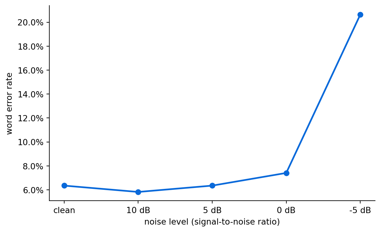
Two findings sit in the table. The phone-band row isolates the codec: stripping every frequency a phone line drops moves the WER far less than heavy noise does in our run, which is one reason modern models transcribe call-center audio usably at all. The noise rows are the curve above, and the curve is the finding, with one caveat: real-world degradation (crosstalk, room echo, compression artifacts) behaves differently from the white noise we synthesized here. The shape, though, is representative. Whisper absorbs light and moderate noise, transcribing perfectly well past the point where the recording would sound rough to a human ear, which is a strength of a modern speech model. But there is a floor, and below it the error rate climbs sharply as the noise overwhelms the words. This is why the WER you trust is the one measured on audio like yours: a model that is flawless on a studio clip can still falter on a phone call recorded from a factory floor, and only your own recordings reveal which regime you are in. The discipline is the same as every other chapter: pick a sample of real recordings, transcribe them, and check the WER against a careful human transcript before you build anything on top.
## Diarization: who said what
To route or analyze a conversation, you also need to know who spoke each line of the transcript. Speaker diarization segments the audio by speaker, labeling stretches as "speaker 1," "speaker 2," and so on, without knowing their names. The standard tool is pyannote. The code is brief, but it requires a multi-speaker recording and a one-time acceptance of the model's terms on Hugging Face, so we show it here without running it.
```{python}
#| eval: false
# Run on a GPU machine, after accepting the model terms and logging in
# with `hf auth login`.
from pyannote.audio import Pipeline

diarizer = Pipeline.from_pretrained("pyannote/speaker-diarization-3.1")
diarization = diarizer(audio_path)

for turn, _, speaker in diarization.itertracks(yield_label=True):
    print(f"{speaker}: {turn.start:.1f}s - {turn.end:.1f}s")
```
The 3.1 pipeline shown here is the established default; pyannote has since released a newer community pipeline that improves on it, and the calling pattern is the same. Diarization gives you time ranges with speaker labels; transcription gives you words with timestamps, and combining them is the step we can run and measure, because our call's true speaker turns are on file. We use those gold turns as the diarization output (on real audio, pyannote produces exactly this list of ranges, with anonymous labels). Granularity is the trap here: Whisper's default segments are long, and a segment that spans a turn boundary assigns every one of its words to one speaker. So for attribution we re-decode with word-level timestamps and place each *word* with whoever held the floor at that moment, merging consecutive same-speaker words back into lines:
```{python}
words = asr(audio_path, return_timestamps="word")["chunks"]

def turn_at(t, turns):
    return next((x["speaker"] for x in turns if x["start"] <= t <= x["end"]), None)

def attribute(words, turns):
    """Label each word by who held the floor, then merge into lines."""
    lines = []
    for w in words:
        t0, t1 = w["timestamp"]
        speaker = turn_at((t0 + (t1 if t1 is not None else t0)) / 2, turns) or "unknown"
        if lines and lines[-1][0] == speaker:
            lines[-1][1].append(w["text"])
        else:
            lines.append([speaker, [w["text"]]])
    return [(spk, "".join(ws).strip()) for spk, ws in lines]

attributed = attribute(words, gold["turns"])
for speaker, text in attributed[:6]:
    print(f"{speaker:9s}| {text[:70]}")
```
And because the script records who truly spoke every word, the result is measurable end to end. The metric is the fraction of the words each speaker actually said that appears, correctly transcribed, in that speaker's attributed transcript. This fraction is one number that transcription errors and attribution errors both pull down, the per-word cousin of diarization error rate (the standard score for how much audio is attributed to the wrong speaker).
```{python}
from collections import Counter

def speaker_bag(pairs):
    bags = {}
    for speaker, text in pairs:
        bags.setdefault(speaker, []).extend(normalize(text))
    return {spk: Counter(ws) for spk, ws in bags.items()}

got = speaker_bag(attributed)
want = speaker_bag([(t["speaker"], t["text"]) for t in gold["turns"]])
correct = sum((got.get(spk, Counter()) & bag).total() for spk, bag in want.items())
total = sum(bag.total() for bag in want.values())
print(f"speaker-attributed word recall: {correct / total:.0%}")
```
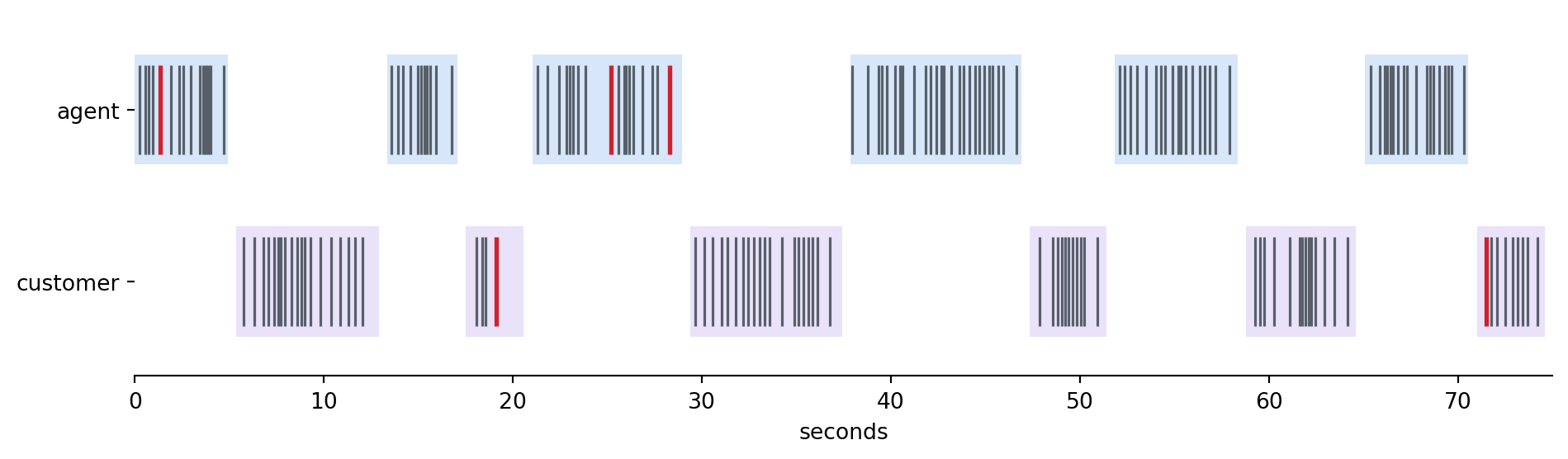
Recall is one number; the timeline below shows where the lost words are. Every transcribed word becomes a tick at its timestamp midpoint, in the lane it was *attributed* to, against the translucent bands of the true speaker turns.
```{python}
#| label: fig-attribution-timeline
#| fig-cap: "Every transcribed word placed on the call's timeline in the lane attribution assigned it, against the translucent bands of the true speaker turns. Gray ticks were attributed to the right speaker; red ticks were not, and they cluster at the edges of the bands, where a word's timestamp drifts across a turn boundary."
#| fig-alt: "Timeline chart from 0 to 75 seconds with two horizontal lanes labeled agent and customer. Translucent blue and purple bands mark each speaker's true turns, short vertical gray ticks mark correctly attributed words inside the bands, and a few red ticks sit near band edges."
def true_speaker(word, turns):
    """The speaker whose nearby gold turn actually contains this word's text."""
    tokens = normalize(word["text"])
    if not tokens:
        return None
    t0, t1 = word["timestamp"]
    mid = (t0 + (t1 if t1 is not None else t0)) / 2
    best, best_dist = None, None
    for turn in turns:
        if tokens[0] in normalize(turn["text"]):
            d = 0.0 if turn["start"] <= mid <= turn["end"] else min(
                abs(mid - turn["start"]), abs(mid - turn["end"]))
            if best_dist is None or d < best_dist:
                best, best_dist = turn["speaker"], d
    return best

lane_y = {"agent": 1.0, "customer": 0.0}
band_color = {"agent": "#0969da", "customer": "#8250df"}

fig, ax = plt.subplots(figsize=(10, 3))
for turn in gold["turns"]:
    y = lane_y[turn["speaker"]]
    ax.broken_barh([(turn["start"], turn["end"] - turn["start"])],
                   (y - 0.32, 0.64), color=band_color[turn["speaker"]],
                   alpha=0.16, linewidth=0)

for w in words:
    t0, t1 = w["timestamp"]
    mid = (t0 + (t1 if t1 is not None else t0)) / 2
    attributed = turn_at(mid, gold["turns"]) or "unknown"
    ok = attributed == true_speaker(w, gold["turns"])
    y = lane_y.get(attributed, 0.5)   # a word that falls in a gap sits between lanes
    ax.vlines(mid, y - 0.26, y + 0.26,
              color="#57606a" if ok else "#cf222e",
              linewidth=1.2 if ok else 2.0)

ax.set_yticks([0.0, 1.0], ["customer", "agent"])
ax.set_xlabel("seconds")
ax.set_xlim(0, 75)
ax.set_ylim(-0.55, 1.55)
ax.spines[["top", "right", "left"]].set_visible(False)
plt.tight_layout(); plt.show()
```
The red ticks are the words the recall number loses, and they concentrate at the edges of the bands, where Whisper's word timestamp drifts just across a turn boundary, plus the occasional misheard word that matches no turn at all. The picture shows what the single number cannot: attribution fails at the handoffs between speakers, while words that sit well inside a turn are attributed correctly.
A transcript where every line is attributed is what you actually want. From here the support call becomes "the customer said X, the agent said Y," which you can route, summarize, or score exactly like the support tickets from the earlier chapters; this is the very ticket from Chapter 2, after all, which arrived there as a written ticket and arrives here by phone. Speech, once transcribed and attributed, rejoins the text pipeline. What the gap contains is exactly the transcription errors we already counted (Breitkart, the digit formatting) plus a few words whose timestamps drift across a turn boundary. Word-level timestamps cost some decoding speed, which is why high-volume pipelines often accept segment-level attribution and its boundary errors; we measured the careful version. And one footnote: we aligned against gold turn boundaries, so this score isolates transcription plus alignment; with pyannote's imperfect boundaries on messy real audio, errors also concentrate at turn changes and overlapping speech, which is why diarization error rate is measured separately.
How imperfect the boundaries can get before attribution suffers is measurable too: we jitter every gold boundary by a random offset, three seeded draws per jitter size, and re-run the same attribution and the same recall.
```{python}
def word_recall(turns) -> float:
    """Speaker-attributed word recall, given a set of speaker turns."""
    got_b = speaker_bag(attribute(words, turns))
    want_b = speaker_bag([(t["speaker"], t["text"]) for t in gold["turns"]])
    hit = sum((got_b.get(spk, Counter()) & bag).total() for spk, bag in want_b.items())
    return hit / sum(bag.total() for bag in want_b.values())

rows = []
for jitter in [0.0, 0.25, 0.5, 1.0]:
    recalls = []
    for seed in range(3):
        rng = np.random.default_rng(seed)
        turns = [{**t, "start": t["start"] + rng.uniform(-jitter, jitter),
                  "end": t["end"] + rng.uniform(-jitter, jitter)}
                 for t in gold["turns"]]
        recalls.append(word_recall(turns))
    rows.append({"boundary jitter": f"+/- {jitter:.2f}s",
                 "mean recall (3 draws)": f"{np.mean(recalls):.0%}"})
pd.DataFrame(rows)
```
The table shows the size of the effect the footnote describes. Small boundary errors (a quarter second or so) barely reduce recall, since most words sit comfortably inside their turns and only the words at the edges are at risk. As the jitter grows toward a full second, the at-risk fringe widens and recall falls in step. This is the slack word-level attribution can tolerate: a diarizer's boundaries need only be tighter than the gaps between words and turns, and this sweep, run on your own audio, tells you how tight that is.
```{mermaid}
%%| echo: false
%%| label: fig-speech-pipeline
%%| fig-cap: "The two halves of speech processing and their merge. Transcription produces the words with timestamps, diarization produces the speaker turns, and aligning the two by time yields the attributed transcript the rest of the text pipeline consumes."
flowchart LR
    audio([recording]) --> tr["transcription, Whisper:<br/>words + timestamps"]
    audio --> di["diarization, pyannote:<br/>speaker turns + time ranges"]
    tr --> merge["align segments<br/>by time"]
    di --> merge
    merge --> outp([attributed transcript:<br/>who said what, when])
```
```{python}
#| echo: false
# Hand the attributed lines, with each turn's start time, to the interactive
# transcript below (online edition only).
transcript_lines, cur = [], None
for w in words:
t0, t1 = w["timestamp"]
mid = (t0 + (t1 if t1 is not None else t0)) / 2
spk = turn_at(mid, gold["turns"]) or "unknown"
if cur is not None and cur["speaker"] == spk:
cur["text"] += w["text"]
else:
if cur is not None:
transcript_lines.append(cur)
start = next((t["start"] for t in gold["turns"]
if t["start"] <= mid <= t["end"]), t0)
cur = {"speaker": spk, "text": w["text"], "start": float(round(start, 2))}
if cur is not None:
transcript_lines.append(cur)
for line in transcript_lines:
line["text"] = line["text"].strip()
ojs_define(call_lines=transcript_lines)
```
::: {.content-visible when-format="html"}
Numbers and timelines aside, the most direct check is to listen. The transcript below is the attributed output itself, with each line showing the speaker the pipeline assigned and the time at which its turn begins.
```{ojs}
//| echo: false
//| label: fig-click-transcript
//| fig-cap: "The attributed transcript, wired to the recording at the top of the chapter. Clicking a line jumps the audio player to the start of that turn, so you can hear the words attribution placed there."
viewof click_transcript = {
  const lines = call_lines;
  const accents = { agent: "#0969da", customer: "#8250df", unknown: "#bf8700" };
  const container = document.createElement("div");
  container.style.cssText = "font-family: inherit; color: var(--bs-body-color, #1f2328); border: 1px solid var(--bs-border-color, #d0d7de); border-radius: 6px; padding: 12px; max-width: 640px;";
  const hint = document.createElement("div");
  hint.style.cssText = "font-size: 12px; color: var(--bs-secondary-color, #57606a); margin-bottom: 8px;";
  hint.textContent = "Click a line to listen from that turn (plays through the audio player at the top of the chapter).";
  container.appendChild(hint);
  lines.forEach(ln => {
    const row = document.createElement("div");
    row.style.cssText = "display: flex; gap: 8px; align-items: baseline; padding: 5px 6px; border-radius: 4px; cursor: pointer; margin: 2px 0;";
    row.onmouseenter = () => { row.style.background = "rgba(128,128,128,0.18)"; };
    row.onmouseleave = () => { row.style.background = "transparent"; };
    row.onclick = () => {
      const player = document.querySelector("audio");
      if (player) { player.currentTime = ln.start; player.play(); }
    };
    const chip = document.createElement("span");
    chip.textContent = ln.speaker;
    const accent = accents[ln.speaker] || "#bf8700";
    chip.style.cssText = `flex: none; font-size: 11px; font-weight: 600; color: ${accent}; border: 1px solid ${accent}; border-radius: 10px; padding: 0 8px;`;
    const stamp = document.createElement("span");
    stamp.textContent = `${ln.start.toFixed(1)}s`;
    stamp.style.cssText = "flex: none; font-size: 11px; color: var(--bs-secondary-color, #57606a); min-width: 40px;";
    const text = document.createElement("span");
    text.textContent = ln.text;
    text.style.cssText = "font-size: 13px;";
    row.append(chip, stamp, text);
    container.appendChild(row);
  });
  return container;
}
```
:::
::: {.content-visible when-format="pdf,epub"}
The online edition links each line of this transcript to its position in the recording. The attributed lines printed above are the same transcript in static form.
:::
::: {.callout-note title="Side note: voice agents"}
By 2026, realtime speech-to-speech agents that can listen and answer in voice without any visible transcript in between have become commonplace in customer support. This chapter deliberately covers the other half: batch transcription, the analytics substrate that turns a recorded call into text you can search, evaluate, and run retrieval-augmented generation (RAG) over. Voice agents are out of scope for this book, but the transcripts this pipeline produces are how you would analyze and evaluate one.
:::
## Evaluation: word error rate on your audio
The evaluation that matters for speech is WER, computed on audio like the audio you will actually process.
**Metric**: word error rate against a human reference transcript.\
**Test set**: a sample of recordings representative of your real audio, because clean studio clips overstate what the model will achieve on your calls.\
**Baseline**: a smaller or older speech model, to see whether a larger one is worth its slower speed.
The trap here is the same one we meet everywhere: a model that scores a low WER on clean benchmark audio can perform far worse on your noisy phone calls, and the only way to know is to measure on your own recordings. Diarization has its own metric, diarization error rate, which scores how much of the audio was attributed to the wrong speaker; when who-said-what matters for your use case, measure that too, because a perfect transcript attributed to the wrong people is still wrong.
::: {.callout-important title="Compliance: recordings are sensitive by default"}
Call recordings are one of the most regulated types of data that a business can have. Many jurisdictions require consent to record, and a recording will contain personal details, voices, and sometimes payment information. Sending this audio to a transcription service, or even processing it on your own machines, is a decision that carries legal weight in most places. Appendix D covers when consent and residency rules apply; for audio they almost always do.
:::
::: {.callout-tip title="Cost: transcription is the cheap step"}
Transcribing audio is inexpensive, whether by API or on your own GPU, and a long call costs a few cents to turn into text; on owned hardware the same statement reads as throughput, with transcription accounting for a small share of the GPU time that the analysis after it consumes. Most of the expense in a speech pipeline sits in what follows the transcription: the summarization, the analysis, the storage of sensitive recordings, and the human review that compliance often requires.
:::
## Exercises
### Conceptual questions
1. Transcription turns audio into words. Diarization adds:
A. Punctuation and casing, which raw speech models leave out of their transcripts
B. A translation of each segment into the language the rest of the pipeline expects
C. Word-level timestamps, so each phrase can be located inside the recording
D. A speaker label for each stretch of audio, so you know who said which part
2. Word error rate measures:
A. How long the model takes to transcribe each minute of recorded audio
B. The fraction of words wrong, counting substitutions, insertions, and deletions
C. The share of a recording's runtime attributed to the wrong speaker after alignment
D. The signal-to-noise ratio below which a transcript stops being usable
3. In the noise experiment, WER stayed low through moderate noise and then climbed steeply at the lowest signal-to-noise ratios. What does this shape show?
A. The model absorbs moderate noise, then fails sharply once the words dissolve into it
B. WER rises in steady proportion to noise, so even light noise costs measurable accuracy
C. The recording was too short for the metric to register errors at moderate noise
D. The pipeline's automatic chunking breaks down once the signal-to-noise ratio drops
4. To evaluate transcription for your own pipeline, the chapter says the test set should be:
A. The clean benchmark clips that the model's developers report their numbers on
B. Synthetic audio with noise added, so the difficulty stays fully under your control
C. A sample of your real recordings, paired with careful human reference transcripts
D. The longest recordings you have, since long audio is the hardest case to chunk
5. An attributed transcript, where every line has a speaker, is produced by:
A. Asking Whisper to identify each distinct voice while it transcribes the recording
B. Aligning transcription segments with diarization turns by their timestamps
C. Prompting a language model to infer the speaker of each line from its content
D. Filtering the audio so that only one speaker's voice remains before transcribing
6. A call transcript can have a perfect WER and still be wrong for your use case because:
A. WER only counts substituted words, so insertions and deletions slip through unscored
B. A low WER on one sample clip guarantees similarly low error across the full recording
C. WER is computed on normalized lowercase text, so it cannot detect any wrong words at all
D. Every line can be attributed to the wrong speaker, which WER never measures
7. Once a call is transcribed and attributed, the chapter's point is that it:
A. Rejoins the text pipeline, ready to be routed, summarized, and searched like a ticket
B. Must remain in audio form for compliance, with the transcript serving as an index
C. Needs a dedicated speech-analytics model before any further analysis can begin
D. Should be re-transcribed with a larger Whisper variant before anything is built on it
8. Why are call recordings treated as especially sensitive data?
A. They are large files whose storage costs come to dominate a pipeline's budget
B. Their transcripts are too unreliable to be admitted in regulated industries
C. Recording often requires consent, and the audio carries voices and personal details
D. Speech models keep a copy of every clip they transcribe unless told otherwise
### Build lab
Transcribe the support call with two Whisper sizes (for example `whisper-tiny` and `whisper-small`) and compare both the WER against the gold script and the time each takes. Report the trade between accuracy and speed, and pick the size you would use for a high-volume call-transcription pipeline.
### Evaluate lab
Apply a proper WER normalizer before scoring: lowercase both sides, spell out or digitize numbers consistently, and strip filler tokens, then recompute the call's WER and report how much of the raw error was formatting and how much reflects genuinely misheard words. Then, if you can accept the pyannote model terms, run real diarization on the call, swap its turns in for the gold ones in the attribution code, and report how the attribution accuracy changes. Decide whether the pipeline is good enough to attribute lines automatically or needs human review.
::: {.callout-note title="Where we go next"}
Speech was the first of the three modalities in this part, and its lesson generalizes: get the signal into text, then reuse everything we already built. In Chapter 19 we apply the same move to images, using a vision-language model to read charts, scanned documents, and product photos into text and structured data.
:::