from dotenv import load_dotenv
load_dotenv()

import pandas as pd10 Context engineering
Deciding what goes into the window, and what to leave out
Paste all eight annual reports into one prompt and ask a question, and the model answers in seconds. You also pay for every token you sent, and the model can still miss a figure that sits on page two. Modern context windows are enormous, hundreds of thousands of tokens, and that size invites misuse. The natural instinct is to fill the window: retrieve twenty chunks where three would do, paste in the whole document, keep the entire conversation history. The instinct is wrong on two counts. Every token costs money, so a full window is an expensive window. And a model’s attention is not uniform across a long context; bury the relevant fact among thousands of irrelevant tokens and the model can miss it. Context engineering is the discipline of deciding what belongs in the window. This chapter shows, with measurement, that more context is usually not better, and that the correct approach is to include the fewest, best tokens that answer the question.
NoteIn the running system
Every prompt our desk sends costs money and competes for the model’s attention, so we keep the document path cheap and accurate. The lesson, the fewest best tokens, applies to triage and the agent as much as to retrieval.
NoteSetup for this chapter
Run in the gaba-core environment with an OPENROUTER_API_KEY. We reuse the report corpus and gaba.rag and gaba.eval from earlier chapters. The corpus embeds once. The distractor stress test (burying the answer among hundreds of irrelevant chunks) sends a few hundred thousand input tokens through the cheap default model, so expect the chapter’s API cost to be a few cents, above the fraction of a cent typical of other chapters.
10.1 The context window is a budget
Although an enormous window can seem like a free resource, two facts make it a budget. The first is cost: you pay per input token, so doubling the context doubles the input bill for every call, though prompt caching (Chapter 2) softens that for a stable prefix that repeats across calls. The second is attention. Research on long contexts keeps finding the same thing: models attend most reliably to the beginning and end of a long input and least reliably to the middle, the “lost in the middle” effect (first measured by Liu and colleagues in 2023 and reproduced widely since). A crucial sentence sitting in the middle of a ten-thousand-token context is at real risk of being overlooked, even though it is technically “in the window.” The picture has improved: today’s frontier models pass simple find-the-fact tests at lengths their predecessors could not handle, but the effect persists in the harder setting, reasoning over many facts spread through a long context. So a full window costs more and can work worse, and both pressures point the same way, toward including less and choosing it better.
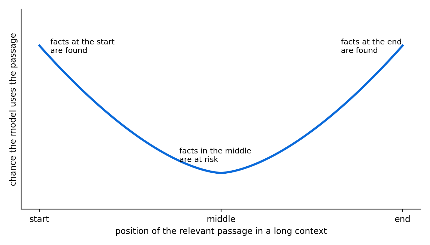
Million-token windows raise a fair question this chapter should answer directly: why retrieve at all, when a small corpus could simply be pasted into the prompt? For a corpus the size of ours, that is a real alternative, and sometimes the right one. It costs more per call, since every question pays for the whole corpus, though caching the corpus as a stable prefix narrows that gap considerably. Retrieval keeps two advantages that do not fade: attribution, because a retrieved chunk tells you where the answer came from in a way a million-token prompt does not, and headroom, because a corpus that grows past any window forces retrieval eventually, so building it early is rarely wasted. Before trusting a model to read the long contexts you plan to give it, run Appendix B’s needle-in-a-haystack test (hiding one fact in a long context and checking the model still finds it) at those lengths.
10.2 The sweet spot has two failure modes
The cleanest way to see the tradeoff is to vary how much context retrieval-augmented generation (RAG) answers get and measure both what they cost and whether they are still complete. One question would make the measurement fragile, so we sweep four questions of different structure: a single-fact question, two questions that each need two facts from one company’s report, and a stretch case whose two facts appear in two different companies’ reports. Each question is answered with the top 1, 2, 4, 8, and 16 retrieved chunks, and the Chapter 9 judge grades completeness.
A keyword check would be free and deterministic, but Chapter 9 taught us what it costs: it is blind to paraphrase, and across four differently phrased questions it would need four hand-tuned patterns. The judge is the check that generalizes.
from concurrent.futures import ThreadPoolExecutor
from gaba.rag import retrieve, RAG_SYSTEM
from gaba.llm import call_llm
from gaba.eval import llm_judge

sweep_questions = {
    "single fact (AMZN)": "What was Amazon's total revenue for 2023?",
    "two facts (AMZN)": ("What were Amazon's total net sales and its operating "
                         "income for the year? Give both figures."),
    "two facts (HRL)": ("What were Hormel's net sales and its operating cash "
                        "flows in fiscal 2023? Give both figures."),
    "two companies": ("What were Amazon's total revenue and Hormel's net sales "
                      "for the most recent fiscal year? Give both figures."),
}
ks = [1, 2, 4, 8, 16]

# The two-fact Amazon question is this chapter's running example; later
# sections reuse its retrieval.
question = sweep_questions["two facts (AMZN)"]
hits_for = {name: retrieve(q, n=16) for name, q in sweep_questions.items()}
all_hits = hits_for["two facts (AMZN)"]

def sweep_one(case):
    name, k = case
    q = sweep_questions[name]
    context = "\n\n".join(f"[{h['ticker']}] {h['text']}" for h in hits_for[name][:k])
    answer = call_llm(f"Context:\n{context}\n\nQuestion: {q}", system=RAG_SYSTEM)
    judged = llm_judge(q, answer.text, context)
    return {"question": name, "chunks": k,
            "input tokens": answer.input_tokens, "complete": judged.complete}

cases = [(name, k) for name in sweep_questions for k in ks]
with ThreadPoolExecutor(max_workers=8) as pool:
    sweep = pd.DataFrame(list(pool.map(sweep_one, cases)))

per_k = (sweep.groupby("chunks")
         .agg(completeness_rate=("complete", "mean"),
              mean_input_tokens=("input tokens", "mean"))
         .round({"completeness_rate": 2, "mean_input_tokens": 0})
         .reset_index())
per_k| chunks | completeness_rate | mean_input_tokens | |
|---|---|---|---|
| 0 | 1 | 0.50 | 246.0 |
| 1 | 2 | 0.75 | 404.0 |
| 2 | 4 | 0.75 | 774.0 |
| 3 | 8 | 0.75 | 1433.0 |
| 4 | 16 | 0.75 | 2870.0 |
The per-k summary shows the budget curve, and the per-question grid below it shows which questions drive it.
sweep.pivot(index="question", columns="chunks",
values="complete").reindex(list(sweep_questions))| chunks | 1 | 2 | 4 | 8 | 16 |
|---|---|---|---|---|---|
| question | |||||
| single fact (AMZN) | True | True | True | True | True |
| two facts (AMZN) | False | True | True | True | True |
| two facts (HRL) | True | True | True | True | True |
| two companies | False | False | False | False | False |
import matplotlib.pyplot as plt

fig, ax = plt.subplots(figsize=(6.5, 4))
ax.plot(per_k["chunks"], per_k["completeness_rate"], color="#0969da",
        marker="o", markersize=8, linewidth=1.5)
for _, r in per_k.iterrows():
    ax.annotate(f"{int(r['mean_input_tokens'])} tok",
                (r["chunks"], r["completeness_rate"]),
                xytext=(0, 12), textcoords="offset points",
                ha="center", fontsize=9, color="#57606a")
ax.set_xlabel("chunks included in the context")
ax.set_ylabel("completeness rate (4 questions)")
ax.set_xticks(per_k["chunks"])
ax.set_ylim(-0.05, 1.15)
ax.spines[["top", "right"]].set_visible(False)
plt.tight_layout()
plt.show()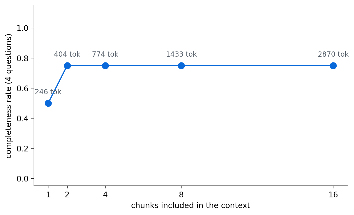
Read the grid by rows, because the rows behave differently, and the difference is the point of sweeping more than one question. The single-fact question is satisfied almost immediately: one good chunk carries its one fact. The two-fact questions expose the first failure mode, starvation: at the smallest contexts the answer carries only what its few chunks happen to contain, one of the figures or even neither, because a grounded system will not invent what it was never shown, and each row fills in only at the depth where retrieval has covered both facts, a depth that differs by question. The two-company question is the stretch case: its facts sit in two different companies’ reports, so it needs the ranked list for a single blended query to surface the right chunk from each company, which is harder than ranking one company’s chunks well, and in our run its row is the one that keeps the rate curve low. If that row never completes at any k, the finding is more useful than any single number: retrieval is the binding constraint for that workload, because no context size fixes a chunk that was never retrieved. The second failure mode is visible in the token annotations: past the plateau, every extra chunk changes nothing but the bill. Too little context starves the answer; too much wastes money and, in a long enough context, risks burying the facts that matter. The sweet spot is the smallest k at the plateau, and because it is a property of your question mix, no single constant serves every workload: a desk that asks single-fact questions and a desk that asks cross-company ones should not settle on the same k, and the grid makes the difference visible.
10.3 Burying the facts: a distractor stress test
The lost-in-the-middle schematic earlier in this chapter is from other people’s research, so we run our own version of the measurement. The two chunks that answer the running two-fact question become the needle, and the haystack is a pile of chunks drawn at random from the other seven companies’ reports. We vary both the size of the pile and where in the pile the two relevant chunks sit: first, buried in the middle, or last. We use three trials per condition, with the judge grading completeness as before.
TipWith an AI coding tool
Assembling the distractor pool, sampling noise chunks per trial, and splicing the two relevant chunks into the first, middle, or last position is mechanical scaffolding, the kind of harness an assistant drafts quickly and well. Read what it hands back for one thing: that the two spliced-in chunks are identical across every condition, so that position and pile size are the only variables the comparison tests. Once that check passes, trust the loop and give your attention to the completeness numbers it produces.
import random
from gaba import DATA_DIR
from gaba.rag import chunk_markdown, REPORTS

# Distractor pool: every company's chunks except Amazon's.
distractor_pool = []
for ticker, filename in REPORTS.items():
    if ticker == "AMZN":
        continue
    for chunk in chunk_markdown((DATA_DIR / "filings" / filename).read_text()):
        distractor_pool.append(f"[{ticker}] {chunk}")

relevant = [f"[{h['ticker']}] {h['text']}" for h in all_hits[:2]]

def bury(condition):
    n_distractors, position, trial = condition
    noise = random.Random(trial).sample(distractor_pool, n_distractors)
    if position == "first":
        blocks = relevant + noise
    elif position == "last":
        blocks = noise + relevant
    else:
        mid = len(noise) // 2
        blocks = noise[:mid] + relevant + noise[mid:]
    context = "\n\n".join(blocks)
    answer = call_llm(f"Context:\n{context}\n\nQuestion: {question}",
                      system=RAG_SYSTEM)
    return {"distractor chunks": n_distractors, "position": position,
            "complete": llm_judge(question, answer.text, context).complete}

conditions = [(n, position, trial)
              for n in [16, 60, 120]
              for position in ["first", "middle", "last"]
              for trial in range(3)]
with ThreadPoolExecutor(max_workers=8) as pool:
    burial = pd.DataFrame(list(pool.map(bury, conditions)))

(burial.pivot_table(index="distractor chunks", columns="position",
                    values="complete", aggfunc="mean")
.reindex(columns=["first", "middle", "last"]))| position | first | middle | last |
|---|---|---|---|
| distractor chunks | |||
| 16 | 1.0 | 1.0 | 1.0 |
| 60 | 1.0 | 1.0 | 1.0 |
| 120 | 1.0 | 1.0 | 1.0 |
The table does not have to show a failure to be informative. If the middle column sags as the pile grows, that is the U curve from the schematic, measured on our own corpus, and the strongest possible argument for curating context. If instead every cell holds at 1.0, the right reading is narrower and still worth having: for this model, at piles up to about a hundred chunks, retrieving two facts succeeds at any placement, which matches where the research has moved, simple fact-finding in long contexts is largely solved, and the degradation now shows up in harder regimes, more facts to hold at once, longer contexts, reasoning across them. Either way the cells are now the claim, since they describe our corpus where the schematic described other people’s, and the method is the deliverable: when your contexts grow past what we tested here, this is the grid to rerun before trusting them. And whatever the positional verdict, the token cost stands: a 120-chunk context pays for 120 chunks on every call, which is the budget argument the next section acts on.
10.4 Curating the context versus dumping it
If a small amount of well-chosen context is what we want, the work lies in the choosing. The single most effective technique combines two tools we already have: retrieve a generous set of candidates, rerank them so the best rise to the top (Chapter 8), and then keep only the few best. You get the recall of a wide retrieval and the precision of a tight context.
from gaba.rag import rerank

# Dump: answer from all 16 retrieved chunks.
dump_context = "\n\n".join(f"[{h['ticker']}] {h['text']}" for h in all_hits)
dump = call_llm(f"Context:\n{dump_context}\n\nQuestion: {question}", system=RAG_SYSTEM)

# Curate: rerank the 16, keep the best 3.
best = rerank(question, all_hits)[:3]
curated_context = "\n\n".join(f"[{h['ticker']}] {h['text']}" for h in best)
curated = call_llm(f"Context:\n{curated_context}\n\nQuestion: {question}", system=RAG_SYSTEM)
Curation can also happen before the ranking, using metadata we already have. In Chapter 6, we stored a ticker on every chunk and promised we would put it to work. Now, when the question names a company, a metadata filter restricts the search to that company’s chunks, so semantic ranking never even receives a cross-company near-miss that could crowd the context.
from gaba.rag import build_corpus
from gaba.embed import embed_texts

qv = embed_texts([question])[0]
res = build_corpus().query(query_embeddings=[qv.tolist()], n_results=3,
                           where={"ticker": "AMZN"})
filtered_hits = [{"ticker": m["ticker"], "text": d}
                 for d, m in zip(res["documents"][0], res["metadatas"][0])]
print("tickers retrieved:", [h["ticker"] for h in filtered_hits])

filtered_context = "\n\n".join(f"[{h['ticker']}] {h['text']}" for h in filtered_hits)
filtered = call_llm(f"Context:\n{filtered_context}\n\nQuestion: {question}",
                    system=RAG_SYSTEM)
tickers retrieved: ['AMZN', 'AMZN', 'AMZN']The three strategies meet in one comparison, where each answer is judged against the context it was actually given.
rows = []
for label, result, ctx in [
    ("dump (16 chunks)", dump, dump_context),
    ("curated (rerank, best 3)", curated, curated_context),
    ("filtered (ticker=AMZN, top 3)", filtered, filtered_context),
]:
    verdict = llm_judge(question, result.text, ctx)
    rows.append({"strategy": label, "input tokens": result.input_tokens,
                 "cost $": round(result.cost_usd, 5),
                 "faithful": verdict.faithful, "complete": verdict.complete})
pd.DataFrame(rows)| strategy | input tokens | cost $ | faithful | complete | |
|---|---|---|---|---|---|
| 0 | dump (16 chunks) | 2919 | 0.00079 | True | True |
| 1 | curated (rerank, best 3) | 583 | 0.00021 | True | True |
| 2 | filtered (ticker=AMZN, top 3) | 609 | 0.00021 | True | True |
The curated answer uses a fraction of the dump’s tokens and stays faithful and complete: we spent a little compute on reranking to save on every answer that follows, and we kept the model’s attention on the passages that matter, where a dump would have diluted it across a dozen near-misses. This is context engineering in a single technique: retrieve wide, rank hard, include little. The filtered row reaches a similarly lean context by a different route, and the two routes have different costs. The reranker spends compute on every query to infer which chunks matter; the filter spends nothing at query time, because the work was done back when we stored a ticker on each chunk. The two mechanisms are complementary: the filter guarantees every candidate is from the right company, a hard constraint embeddings can only approximate, and semantic ranking orders chunks within that guarantee. Filters pay off wherever the corpus has structure the query can name, a company, a year, a document type, and a question that names two companies simply needs one filtered search per company.
Two more techniques belong in the toolkit, and both matter most once we reach the multi-turn agents of Part IV. Summarization checkpoints: when a conversation or a chain of steps grows long, periodically replace the old turns with a short summary, so that the running context stays small where it would otherwise grow without bound. Scratchpads: give the model a place to write down intermediate results and pull them back when needed, so that the prompt need not carry everything. Both are the same idea as curation, applied across time where it was earlier applied across documents: keep what is needed in the window, and move the rest out.
flowchart TB
    subgraph checkpoint["Summarization checkpoint: compress the past"]
        old["Turns 1 to 8<br/>(growing history)"] --> summ["Short summary"]
        summ --> win["Window: summary<br/>+ recent turns only"]
        recent["Turns 9 to 12"] --> win
    end
    subgraph scratch["Scratchpad: park results outside the window"]
        stepA["Step writes an<br/>intermediate result"] --> padfile["Scratchpad<br/>(outside the window)"]
        padfile --> stepB["A later step reads it back<br/>only when needed"]
    end
    checkpoint ~~~ scratch
10.5 Evaluating the choice of context size
The sweep above is the evaluation, and it answers a real design question: how much context should this system use? The method generalizes.
Metric: answer completeness and faithfulness (the Chapter 9 judge), paired with cost per answer.
Test set: questions answerable from the corpus, mixed to match real traffic: single-fact, multi-fact, and cross-document.
Baseline: the most-context option, which is the one a team would reach for by default.
You run the sweep on a question mix that matches your real traffic, find the smallest context size where the completeness rate reaches its plateau, and use that size. In our sweep the per-question grid shows which questions settle early and which delay the plateau, the per-workload lesson in miniature. On a harder corpus, or a more demanding question mix, the sweet spot sits further right, and the only way to know is to measure, because a guess has no evidence behind it. There are two mistakes to avoid, and they point in opposite directions. The first is the reassuring default, “include everything just in case,” which is the most expensive option and, thanks to lost-in-the-middle, not even reliably the most accurate. The second is starving the context to save a few cents, which delivers an answer that is quietly incomplete. The sweep is how you avoid both.
TipCost: manage the context first
For most large language model (LLM) applications the input context dominates the bill, because the prompt is long and the answer is short. That makes context the most effective place to manage cost. Halving the chunks you include roughly halves the input cost of every call, forever, and as we just measured it often costs you nothing in quality. Self-hosted, the same halving appears as latency and throughput: fewer input tokens per call means less prefill work, so the same hardware serves more questions. Before switching to a cheaper model, examine how many tokens you are placing in the window.
The sweep’s token counts turn this callout into arithmetic you can do for your own workload. Below is a calculator to price a month of answers using the input tokens we measured at each context size. Set the chunks per answer, the monthly question volume, and the input price of your model, and compare the bill against dumping all sixteen chunks.
WarningDon’t outsource this
An assistant can write the retrieval and reranking code, but it cannot decide how much context your system should carry, because that decision is a measured tradeoff between cost and faithfulness on your data: run the sweep, read the curve, and pick the point yourself.
10.6 Choosing your retrieval and evaluation stack
Part III added a reranker, weighed hybrid search, and built the evaluation toolkit. The tools below are where those techniques come from.
| Capability | Open-weight | Hosted | Choose by |
|---|---|---|---|
| Reranking | BGE reranker v2-m3, Jina, mixedbread | Cohere Rerank, Voyage | running it locally against an API |
| Keyword and hybrid | rank_bm25, Elasticsearch, OpenSearch | managed search services | corpus size and filtering needs |
| Evaluation | Ragas, DeepEval, promptfoo | Phoenix, LangSmith, Braintrust | a library you run against a hosted dashboard |
Important
- Measure before adding any of these. On an easy corpus, the plain retriever is often already at the ceiling (Chapter 8).
- Rerank only a shortlist, since the cross-encoder is too slow to read the whole corpus (Chapter 8).
- Pin the judge model and version, and validate it against human labels before trusting its scores (Chapter 9).
Common failure points
- Trusting an automated judge you never checked, so the metric is confidently wrong (Chapter 9).
- Optimizing a retrieval metric that does not match what is at stake for the business (Chapter 9).
- Adding hybrid search or query rewriting blindly, paying for complexity that adds nothing (Chapter 8).
The current open-source and vendor options for these are in the tooling-landscape appendix, dated and fuller; model and provider choice is Appendix E.
10.7 Exercises
10.7.1 Conceptual questions
Why do we treat a large context window as a budget, even though it appears to be a free resource?
- Providers cap the number of calls per day in proportion to window size
- Every token costs money, and attention degrades over long contexts
- Longer inputs force the model to produce proportionally longer answers
- The usable window shrinks steadily as a conversation grows longer
In the sweep, answers were incomplete at the smallest contexts, became complete once enough chunks were included, and beyond that point only the bill grew. The lesson is:
- A sweet spot exists: too little context starves the answer, more only adds cost
- Sixteen chunks would have been the safe choice, since cost is secondary
- One chunk is the right default, and the failure there was the checker’s
- Completeness keeps rising with context, so the trend continues past sixteen
The “lost in the middle” effect means a model is most likely to overlook information placed:
- In the system prompt, which models treat as optional guidance
- At the very start of a long context
- At the very end of a long context
- In the middle of a long context, far from either edge
Starved of context, the two-fact Amazon answer reported net sales but omitted operating income. Why?
- The model exhausted its output token limit before the second figure
- The completeness check failed to recognize the figure in the answer
- That figure sat in a chunk the model never saw, and a grounded system will not invent it
- Operating income was in the shown chunk, but lost-in-the-middle hid it
“Retrieve wide, rank hard, include little” combines which two tools?
- Wide retrieval for recall and reranking for precision, then a small context
- Hybrid keyword search with query rewriting, feeding a larger context
- Two different embedding models voting on which chunks deserve to stay
- Summarization checkpoints paired with a scratchpad for intermediate results
In the chapter’s evaluation of context size, why is the most-context option the baseline?
- It is guaranteed to produce the most faithful answers, so it sets the ceiling
- The judge needs all sixteen chunks in order to grade any answer at all
- A baseline must always be the most expensive option in the comparison
- It is the default a team would reach for, so it is the option to beat
Summarization checkpoints and scratchpads apply the idea of curation:
- To the output side of the call, trimming the answers the model returns
- Only to single-turn questions, since agents cannot make use of summaries
- Across time, keeping the running context small as a conversation grows
- To the embedding step, by compressing vectors into fewer dimensions
For most LLM applications, which part of the bill dominates?
- The output tokens, since generation is the expensive direction
- Input tokens, because prompts are long and answers are short
- The embedding calls that turn the corpus and queries into vectors
- The vector database serving nearest-neighbor lookups at query time
10.7.2 Build lab
Add three questions of your own to the chapter’s sweep, matched to your idea of real traffic, including at least one whose facts span two chunks. Recompute the per-k completeness rate and the per-question grid. Report the smallest chunk count where completeness holds across your additions, and the monthly cost saving versus sixteen chunks for a 50,000-question desk. You may use an assistant for the loop, but you decide what “holds” means.
10.7.3 Evaluate lab
The chapter’s two-company question forces one blended query to surface the right chunk from each of two companies, and the per-question grid shows how that went. Build the fix the metadata-filter section pointed at: detect the two companies in the question, run one filtered search per company, and merge the top chunks into a single context to answer the question. Measure completeness across several k values for your fix and for the blended-query baseline. Report whether splitting the retrieval beat enlarging the context, with the numbers that say so.
TipProject ideas
You can now measure retrieval quality, build a golden set, and improve answers with reranking, query rewriting, and a context budget. With these two projects, you can turn that into a habit of measure-then-change.
- Measure and improve a RAG system you built. Take the assistant from Part II, write a golden set of questions with known answers, and score retrieval with precision@k before and after each change: add a reranker, rewrite queries, switch to hybrid search. Keep the changes that move the number and drop the ones that do not. Data to try: your Part II corpus with a hand-written golden set, or a ready benchmark such as BEIR, SQuAD, or HotpotQA.
- A judge you can trust. Build a model-as-judge that grades answers for faithfulness and relevance against the retrieved context. Check the judge against your own labels on a sample before you rely on it. Data to try: a public question-answering set such as MS MARCO or HotpotQA, or answers from your own RAG system.
The discipline here carries into every later part: anything you build from now on, you can measure.
NoteWhere we go next
That closes Part III. We can now retrieve well, answer in a grounded manner, measure everything, and keep the context lean. So far every system has done one thing per model call. In Part IV, the systems start to act: in Chapter 11, we build workflows that chain and route model calls, and in Chapter 12, we turn these workflows into agents that choose their own tools.