from dotenv import load_dotenv
load_dotenv()

from gaba.graph import build_knowledge_graph

G = build_knowledge_graph()
print(f"knowledge graph: {G.number_of_nodes()} nodes, {G.number_of_edges()} edges")
knowledge graph: 32 nodes, 37 edgesAnswering questions that connect facts across documents
Some questions cannot be answered from any single passage. For example, “Who competes with the company that supplies Kestrel Motors’ batteries” needs the supplier from one news story and that supplier’s competitor from another, and no document holds both. Flat retrieval-augmented generation fetches the chunks nearest a question and judges each on its own, so it can answer only when the whole answer sits in one passage. This is a multi-hop question, and it is what the knowledge graph from the last chapter is designed to address.
Graph RAG answers a question by traversing the graph to gather the connected facts, then handing them to a model. In this chapter we build it, walk it through supplier chains, board connections, and shortest paths, and then measure it head to head against flat RAG on the same corpus, because “the graph helps” is a claim that has to be tested.
Run in the gaba-core environment with an OPENROUTER_API_KEY. We reuse gaba.graph from Chapter 21, which builds the knowledge graph once.
from dotenv import load_dotenv
load_dotenv()
from gaba.graph import build_knowledge_graph
G = build_knowledge_graph()
print(f"knowledge graph: {G.number_of_nodes()} nodes, {G.number_of_edges()} edges")knowledge graph: 32 nodes, 37 edgesGraph RAG replaces “embed the question and fetch nearby chunks” with “find the entities in the question and gather the facts connected to them.”
flowchart TB
  Q[Question] --> E[Find entities in the graph]
  E --> T[Traverse edges,<br/>gather connected facts]
  T --> C[Facts as context]
  Q --> P[Prompt: facts plus question]
  C --> P
  P --> L[Language model]
  L --> A[Answer connecting the facts]
The crucial step is the traversal. Starting with the entities named in the question, we walk outward a few hops, collecting every edge we pass. These edges are the facts the model gets, and since they are connected, the model can reason across them.
Two functions in gaba.graph do the work. gather_facts traverses the graph from a set of entities, while graph_rag finds the entities in the question, collects their facts, and answers from them.
from gaba.graph import gather_facts

# The facts within two hops of Kestrel Motors: its own edges, and the edges
# of whatever it connects to.
facts = gather_facts(G, ["Kestrel Motors"], hops=2)
for s, r, o in sorted(facts):
    print(f"  {s} -[{r}]-> {o}")
Aurora Cell Works -[SUPPLIES_TO]-> Juniper Grid
Aurora Cell Works -[SUPPLIES_TO]-> Kestrel Motors
Helio Capital -[INVESTS_IN]-> Aurora Cell Works
Mara Voss -[BOARD_MEMBER_OF]-> Kestrel Motors
Mara Voss -[BOARD_MEMBER_OF]-> Northwind Systems
Pacific Crest Logistics -[ACQUIRED]-> Jonas Kim's earlier startup
Pacific Crest Logistics -[FOUNDED]-> Kestrel Motors
Pacific Crest Logistics -[SUPPLIES_TO]-> Cascadia Foods
Pacific Crest Logistics -[SUPPLIES_TO]-> Saltbox Retail Group
Tomas Okafor -[CEO_OF]-> Kestrel Motors
Voltaic Dynamics -[COMPETES_WITH]-> Aurora Cell WorksStarting with Kestrel Motors, the first hop finds its battery supplier, Aurora Cell Works, from one document. The second hop finds Voltaic Dynamics, Aurora’s competitor, from a different document that never once mentions Kestrel. The traversal also picked up Mara Voss and, through her board seats, Northwind Systems. These second-hop connections are what a flat retriever, fetching documents independently, never assembles.
Reach comes at a cost that is easy to measure, because traversal makes no API calls: each extra hop multiplies the facts gathered, and the facts become the context the answering call must carry.
import pandas as pd
hop_rows = []
for hops in [1, 2, 3]:
facts_h = gather_facts(G, ["Kestrel Motors"], hops=hops)
context = "\n".join(f"{s} {r} {o}" for s, r, o in sorted(facts_h))
hop_rows.append({"hops": hops, "facts gathered": len(facts_h),
"approx context tokens": int(len(context.split()) * 1.3)})
pd.DataFrame(hop_rows)| hops | facts gathered | approx context tokens | |
|---|---|---|---|
| 0 | 1 | 4 | 28 |
| 1 | 2 | 11 | 85 |
| 2 | 3 | 25 | 187 |
On a graph this small, three hops sweeps in most of the ecosystem, and on a production graph the growth is steeper: each hop multiplies the frontier (the nodes reached so far) by the average degree (how many edges a typical node has), so hop counts behave like a context budget. Two hops covers the question types this chapter addresses, supplier-of-supplier, connector-between-companies; deeper questions need either a bigger budget or a smarter traversal that follows only promising edge types. The hop count is the same retrieval trade-off as Chapter 7’s top-k, except that its units are hops and every increment compounds.
Now the full pattern, on three questions of increasing reach. First, the supplier-chain question that opened the chapter:
from gaba.graph import graph_rag
answer, used = graph_rag("Who competes with Kestrel Motors' battery supplier?", G)
print(answer)Kestrel Motors' battery supplier is Aurora Cell Works. Voltaic Dynamics competes with Aurora Cell Works. Therefore, Voltaic Dynamics competes with Kestrel Motors' battery supplier.Second, the connector question, the kind a due-diligence analyst asks: which person links two companies?
answer, used = graph_rag(
"Which board member connects Northwind Systems and Kestrel Motors?", G)
print(answer)Mara Voss connects Northwind Systems and Kestrel Motors.And third, a pure graph operation that needs no model at all: the shortest path between two entities that have, on the surface, nothing to do with each other. How does a hotel chain connect to a robotics company?
import networkx as nx
path = nx.shortest_path(G.to_undirected(), "Tidewater Hotels", "Bluepeak Robotics")
print(" -> ".join(path))Tidewater Hotels -> Granite Bank -> Jonas Kim -> Orchard Software -> Northwind Systems -> Meridian Semiconductors -> Bluepeak RoboticsThe path goes through the hotel chain’s bank, the bank’s former board member Jonas Kim, his company Orchard, Orchard’s acquirer Northwind, and Northwind’s chip supplier Meridian, who also supplies Bluepeak. This is a chain of exposure that no document states and no embedding ever retrieves, computed in a millisecond. The path also records an extraction failure: the text states a shorter route (Tidewater buys its analytics directly from Northwind), but the extractor rendered that fact as a mangled edge, so the three-hop route is absent from the graph and the traversal found the six-hop path. The graph you query is the graph you extracted, which can diverge from the graph the text states, and this divergence is why Chapter 21’s evaluation comes first.
Each of these answers assembled facts from documents that never mention each other. Flat retrieval finds relevant text, while graph retrieval finds connected facts.
flowchart TB
subgraph f["Flat RAG: documents retrieved independently"]
direction LR
qf(["Who competes with Kestrel's<br/>battery supplier?"]) --> ca["doc about Kestrel<br/>and Aurora"]
qf --> cb["doc about Voltaic<br/>and Aurora"]
ca -. "the link through Aurora is<br/>left for the model to notice" .- cb
end
subgraph g2["Graph RAG: facts gathered by traversal"]
direction LR
qg(["same question"]) --> kst(("Kestrel<br/>Motors"))
kst -- "supplied by" --> aur(("Aurora<br/>Cell Works"))
aur -- "COMPETES_WITH" --> vlt(("Voltaic<br/>Dynamics"))
end
f ~~~ g2
One implementation caveat: graph_rag finds the question’s entities by matching node names and the alias table from Chapter 21, longest names first. This handles “Kestrel” finding “Kestrel Motors”, but it is still string matching, and on real graphs, where thousands of entity names vary and collide with common words, a production system uses entity recognition (spotting names of people, places, and organizations in text) to pick the starting nodes. The traversal that follows is unchanged.
“The graph helps with multi-hop questions” is a claim, and to test it we compare Graph RAG head to head with flat RAG built over the same fourteen documents, asked the same questions, and scored the same way.
Metric: fraction of questions whose answer mentions every expected entity.
Test set: five questions, two single-fact (one document holds the answer) and three cross-document multi-hop (the answer requires connecting at least two documents).
Baseline: flat RAG retrieving the top two documents by embedding similarity, the strongest simple version of Chapter 7’s pipeline on this corpus.
The flat_rag function is Chapter 7’s retrieve-then-answer pattern in miniature: embed the question, rank documents by cosine similarity, and concatenate the top k. It is fast and safe to let an assistant draft. Read it for the one choice that decides whether the comparison below is fair: that k is set to the same top-two documents you would actually use in production. A baseline padded with a generous k would make Graph RAG’s multi-hop advantage look larger than it is.
import numpy as np
import pandas as pd
from gaba.embed import embed_texts
from gaba.graph import load_documents
from gaba.llm import call_llm
docs = load_documents()
doc_vecs = embed_texts(docs)
def flat_rag(question: str, k: int = 2) -> str:
"""Chapter 7's pattern in miniature: retrieve top-k documents, answer."""
q_vec = embed_texts([question])[0]
top = np.argsort(doc_vecs @ q_vec)[::-1][:k]
context = "\n\n".join(docs[i] for i in top)
return call_llm(
f"Context:\n{context}\n\nQuestion: {question}",
system="Answer using only the context. If it does not contain the "
"answer, say so.").text
cases = [
# single-fact: one document states the answer
("Who is the chief executive of Meridian Semiconductors?", ["raman"], "single-fact"),
("Which company acquired Orchard Software?", ["northwind"], "single-fact"),
# cross-document multi-hop: the answer spans documents
("Who competes with Kestrel Motors' battery supplier?", ["voltaic"], "multi-hop"),
("Who supplies chips to the company that acquired Orchard Software?",
["meridian"], "multi-hop"),
("Through which companies is Tidewater Hotels connected to Bluepeak Robotics?",
["northwind", "meridian"], "multi-hop"),
]
rows = []
for q, expected, kind in cases:
flat = flat_rag(q).lower()
graph = graph_rag(q, G)[0].lower()
rows.append({"question": q[:48], "type": kind,
"flat RAG": all(e in flat for e in expected),
"graph RAG": all(e in graph for e in expected)})
pd.DataFrame(rows)| question | type | flat RAG | graph RAG | |
|---|---|---|---|---|
| 0 | Who is the chief executive of Meridian Semicondu | single-fact | True | True |
| 1 | Which company acquired Orchard Software? | single-fact | True | True |
| 2 | Who competes with Kestrel Motors' battery suppli | multi-hop | False | False |
| 3 | Who supplies chips to the company that acquired | multi-hop | False | True |
| 4 | Through which companies is Tidewater Hotels conn | multi-hop | False | True |
import matplotlib.pyplot as plt
kinds = ["single-fact", "multi-hop"]
x = np.arange(len(kinds))
fig, ax = plt.subplots(figsize=(6, 3.8))
for offset, (system, color) in zip([-0.18, 0.18],
[("flat RAG", "#cf222e"), ("graph RAG", "#0969da")]):
rates = [np.mean([r[system] for r in rows if r["type"] == kind]) for kind in kinds]
bars = ax.bar(x + offset, rates, width=0.36, color=color, label=system)
ax.bar_label(bars, fmt="%.2f", padding=2, fontsize=8)
ax.set_xticks(x, [f"{kind} (n={sum(r['type'] == kind for r in rows)})" for kind in kinds])
ax.set_ylabel("pass rate")
ax.set_ylim(0, 1.15)
ax.legend(frameon=False)
ax.spines[["top", "right"]].set_visible(False)
plt.tight_layout(); plt.show()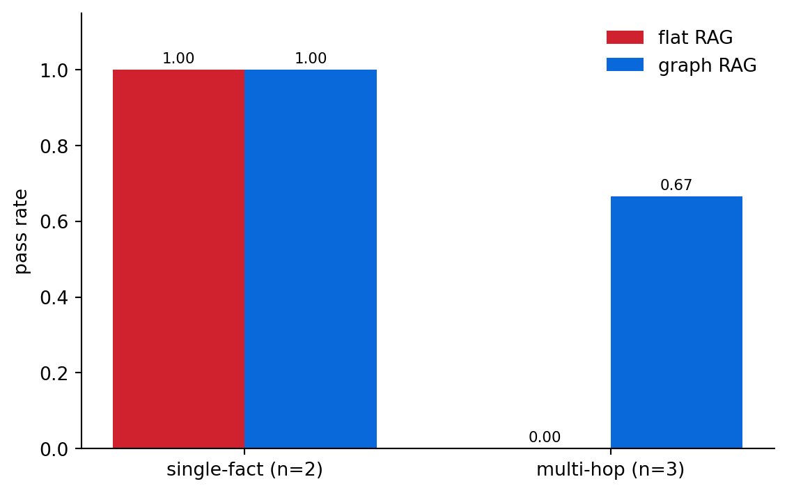
Read the table by row type. On single-fact questions the two systems should tie: when one document holds the answer, similarity search finds that document, and the graph adds nothing. The multi-hop rows are where they separate, and why they separate matters more than the score: flat RAG fails a multi-hop question when the top-k documents do not happen to include every link in the chain, and on a corpus of fourteen documents chance retrieval is common, because two documents out of fourteen is a wide selection. At fourteen thousand documents that chance disappears; the chain’s links are buried under thousands of similar-sounding passages, while the graph traversal follows the chain directly, at a cost set by the number of hops and the graph’s degree, independent of the size of the corpus. If flat RAG happens to pass a multi-hop row here, the pass reflects this small-corpus effect and says nothing about how the system would fare at scale.
When a graph row fails, trace it before concluding the graph is at fault: either the edge was never extracted (Chapter 21’s lesson), or the facts were gathered and the answering model failed to chain them, which the printed fact list makes visible; the two failures have different fixes, a better extractor versus a better answering prompt. The trace is cheap enough to run on the spot. We take the supplier-competitor question, the chapter’s opening example, and print exactly what the answering model was given, however its row came out above.
question = "Who competes with Kestrel Motors' battery supplier?"
answer, facts = graph_rag(question, G)
print("facts handed to the model:")
for s, r, o in sorted(facts):
print(f" {s} -[{r}]-> {o}")
print("\nanswer:", answer)facts handed to the model:
  Aurora Cell Works -[SUPPLIES_TO]-> Juniper Grid
  Aurora Cell Works -[SUPPLIES_TO]-> Kestrel Motors
  Helio Capital -[INVESTS_IN]-> Aurora Cell Works
  Mara Voss -[BOARD_MEMBER_OF]-> Kestrel Motors
  Mara Voss -[BOARD_MEMBER_OF]-> Northwind Systems
  Pacific Crest Logistics -[ACQUIRED]-> Jonas Kim's earlier startup
  Pacific Crest Logistics -[FOUNDED]-> Kestrel Motors
  Pacific Crest Logistics -[SUPPLIES_TO]-> Cascadia Foods
  Pacific Crest Logistics -[SUPPLIES_TO]-> Saltbox Retail Group
  Tomas Okafor -[CEO_OF]-> Kestrel Motors
  Voltaic Dynamics -[COMPETES_WITH]-> Aurora Cell Works
answer: The facts do not contain the answer to this question.The fact list settles the diagnosis: the full chain is present, Aurora Cell Works supplies Kestrel Motors and Voltaic Dynamics competes with Aurora, so retrieval succeeded. If the answer above (or the table’s row for this question) misses Voltaic Dynamics anyway, the failure happened in the answering call, the model declining to chain two facts sitting side by side in its context. The fix, since the graph already delivered the chain, is a better answering prompt or a stronger model. If it names Voltaic Dynamics, the same trace is the diagnostic to run when the pipeline eventually does fail.
Either way, the result deserves limited confidence: a single-run boolean on five questions is a noisy instrument, where one flipped answer moves a pass rate by a third of a bar, and a real harness re-asks each question several times and reports rates with the sample sizes attached, exactly the discipline Chapter 9 built.
The caveats are the ones from Chapter 21: Graph RAG works only as well as the graph is complete, and a relationship the extractor missed is a question it cannot answer no matter how well it traverses. Because these two chapters form one pipeline whose weakest link is extraction, the precision-and-recall evaluation from the last chapter is the one that matters most.
In production the choice is a routing decision. Following the pattern from Chapter 11, a one-line classifier in front dispatches each question to the retriever built for its type: questions about specific entities and their connections go to the graph, while questions asking what a document says go to flat retrieval.
What we built is local Graph RAG: start from the entities in the question and traverse their neighborhood. This serves questions about specific entities and their connections. A different class of question is global, “what themes run across this corpus,” where no entity neighborhood holds the answer. The established approach for such questions is to detect communities in the graph (clusters of densely connected nodes) and build hierarchical summaries of them, the design popularized as Microsoft GraphRAG (Microsoft’s open-source library for community-based graph retrieval). In production the choice is rarely either-or, since most systems combine vector search (for finding relevant text) with graph traversal (for connecting facts).
The graph traversal is pure in-memory computation, both free and instantaneous. Graph RAG’s only model call is the final answer, the same single call a flat RAG answer costs. So Graph RAG is no more expensive at query time than ordinary RAG, since the additional cost was paid once, at indexing time, to build the graph. On owned hardware the same reading holds: traversal consumes no model capacity, so each query costs one generation’s worth of latency and throughput either way. For multi-hop questions you obtain a better answer at the same per-query price.
In Part VIII we extracted a graph from text and answered multi-hop questions over it. The tools are a place to store the graph and a way to build and query it with a model.
| Capability | In-memory or embedded | Server | Choose by |
|---|---|---|---|
| Graph store | NetworkX, Kùzu | Neo4j, Memgraph, ArangoDB | a prototype against persistent scale |
| Graph RAG | LlamaIndex property graph | Microsoft GraphRAG, Neo4j GraphRAG | corpus size and pipeline needs |
Important
Common failure points
The current open-source and vendor options for these are in the tooling-landscape appendix, dated and fuller; model and provider choice is Appendix E.
A multi-hop question is one that:
Why does flat RAG struggle with “who competes with Kestrel Motors’ battery supplier”?
In Graph RAG, the traversal step produces:
Starting from Kestrel Motors, a two-hop traversal reaches Voltaic Dynamics because:
The weakest link in the Graph RAG pipeline is usually:
The chapter flags the entity finding in graph_rag as fragile on real graphs because:
Why is flat RAG over the same fourteen documents the right baseline for the evaluation?
At query time, how does Graph RAG’s cost compare with flat RAG’s?
Observe how the answer changes when you call graph_rag with hops=1 and with hops=2. Since the supplier-competitor question needs two hops, confirm that one-hop traversal fails on it while two-hop traversal succeeds. Then add a document to assets/data/kg/news_snippets.json that creates a genuine three-hop chain (delete the triples cache so the graph rebuilds), and show that three-hop traversal is needed to answer a question about that chain. Report the trade-off between reach and the amount of irrelevant context gathered as the number of hops increases.
Write five multi-hop questions over the graph, three answerable and two whose answer is not in the graph at all. Run Graph RAG on all five and check that it answers the answerable questions and declines the unanswerable ones. Report the two rates separately, the same answer-and-abstain split you measured for flat RAG in Chapter 7.
You can now pull entities and relationships out of text, assemble them into a knowledge graph, and answer multi-hop questions that flat retrieval struggles with. These two projects build a graph and then put it to work.
Part IX turns to what it takes to run any of this in production.
This closes Part VIII, and with it the building of capabilities: every part so far added something the system can do. In Part IX, we turn to making those systems safe to deploy. Chapter 23 defends against prompt injection and the other ways a system that reads untrusted input can be turned against you.