from dotenv import load_dotenv
load_dotenv()

import numpy as np
import pandas as pd
import matplotlib.pyplot as plt8 Advanced retrieval
Reranking, contextual retrieval, and the discipline of measuring first
The basic retrieval-augmented generation (RAG) system from Chapter 7 retrieves by nearness alone: it embeds the query and takes the chunks whose vectors sit closest. Nearness is a rough proxy for relevance, so the system often returns passages that share the question’s words without holding its answer. Search the internet for how to improve RAG and you will be handed a menu of upgrades: rerank the results, add keyword search alongside the vectors, rewrite the query, prepend context to every chunk before embedding. Each is a real technique with a real cost, and each is worth adding only if it helps your system. This chapter does two things at once. It shows what these techniques are and how they work, and it makes the case, with our own numbers, that the right first move is to measure whether they help at all. The common mistake is to add them blindly. On an easy corpus the answer is often no, and knowing that saves you from paying for complexity that adds nothing; on a hard one the answer is a clear yes, and the same measurement tells you so. We will see both, on the same techniques, and the only thing that ports between the two is the habit of measuring. We are still at the retrieve-and-ground stage of the Chapter 1 lifecycle, now improving its accuracy.
NoteIn the running system
This is where our desk’s document answers move from plausible to reliable. The reranking and contextual-retrieval techniques here are upgrades to the Chapter 7 path, applied only after we measure that they help.
NoteSetup for this chapter
Run in the gaba-core environment with an OPENROUTER_API_KEY. We reuse the eight-report corpus and gaba.rag from Chapters 6 and 7, and add gaba.rag.rerank. The first run downloads the reranker model (about 2 GB) from Hugging Face; later runs load it from the local cache. Embedding the corpus twice (plain and contextual) takes a couple of minutes on CPU.
8.1 Tools in this chapter
| Tool | Why we use it here | Alternatives | Trade-off |
|---|---|---|---|
| BGE Reranker v2-m3 | a cross-encoder that rescores a shortlist by reading the query and each chunk together | Cohere Rerank, Jina, mixedbread (hosted or open) | sharper ranking against extra time per query |
Part III closes, in Chapter 10, with the retrieval stack; the tooling-landscape appendix lists the current options.
8.2 Reranking
Our embedding model is a bi-encoder: it turns the query into a vector and each chunk into a vector, separately, and compares them, which is fast, because we embed the chunks once and reuse them forever, but blunt, because the query and the chunk never meet. A cross-encoder reads the query and a chunk together and scores how well they match. It is far too slow to run over a whole corpus, but it is excellent for re-scoring a short list. So the pattern is: retrieve a generous top-k with the fast bi-encoder, then rerank those few with the sharp cross-encoder.
%%{init: {"flowchart": {"subGraphTitleMargin": {"top": 4, "bottom": 28}}}}%%
flowchart TB
    subgraph bi["Bi-encoder: fast, runs over the whole corpus"]
        bq["Query"] -->|"embed separately"| bv["Query vector"]
        bd["Chunk"] -->|"embed separately"| bw["Chunk vector"]
        bv --> cs["Cosine similarity"]
        bw --> cs
    end
    subgraph cross["Cross-encoder: slower, reranks a shortlist only"]
        cq["Query"] --> ce["One model reads<br/>query and chunk together"]
        cd["Chunk"] --> ce
        ce --> sc["Relevance score"]
    end
    bi ~~~ cross
from gaba.rag import retrieve, rerank

query = "How many vehicles were delivered in 2023?"
hits = retrieve(query, n=6)            # fast bi-encoder retrieval
ranked = rerank(query, hits)           # sharp cross-encoder rescoring

print("cross-encoder relevance scores, best first:")
for h in ranked:
    print(f"  {h['rerank_score']:.3f}  [{h['ticker']}] {h['text'][:65]}")
cross-encoder relevance scores, best first:
0.485 [ATSG] Our commitment to innovation and growth remains unwavering. We ex
0.262 [TSLA] We currently manufacture five different consumer vehicles – the M
0.230 [AMZN] We also continue to improve delivery speeds, breaking multiple co
0.081 [ATSG] Looking ahead to 2024, we anticipate a decline in both growth and
0.014 [ATSG] Bundled aircraft leasing, airline solutions, engine power, aircra
0.004 [BAC] In 2023 we also shared our success with those who have so ably seThese scores need careful reading. Cross-encoder outputs are not probabilities, so the absolute numbers mean little on their own; the ordering and the spread between the top chunk and the rest carry the signal. Here the question asks for a specific figure, and the reranker’s job is to pull the passage that reports the delivery number above the chunks that merely talk about vehicles. A wide spread means it has a confident preference; a narrow one, near-zero scores all the way down, means it barely has a preference at all, which is common on an easy corpus where the bi-encoder’s shortlist was already fine. Either way, the lesson is the same one this chapter keeps repeating: you learn which case you are in by reading the numbers, because the technique’s reputation carries no information about your corpus. This run shows why the reading matters: the top-scored chunk is a generic strategy passage from the wrong company, and none of the six candidates contains a delivery figure, because the indexed front portion of each report (Chapter 6’s chunk cap) never included one. A reranker can only reorder what retrieval hands it; when the answer is missing from the shortlist, even a perfect reranker returns the least-wrong miss. The broader point, that pipeline stages cannot be judged in isolation, runs through the chapter: whether reranking changes anything end to end is a question we will answer by measurement.
8.3 Contextual retrieval
Here is a failure that embeddings have by construction: when we chunk a document into small pieces, each piece loses the context of the whole. A chunk that reads “Net sales increased 11% to $574.8 billion” is perfectly clear in Amazon’s report and perfectly anonymous on its own: nothing in those words says Amazon. A query that names the company may then fail to find it, because the company’s name is not in the chunk.
Contextual retrieval, introduced by Anthropic in 2024, fixes this by prepending a short context to each chunk before embedding it, so that the chunk carries its own provenance. In its full form, this context is written by a language model for each chunk, while the cheap version that captures most of the benefit simply prepends the document’s identity.
from gaba.rag import chunk_markdown, REPORTS
from gaba.embed import embed_texts
from gaba import DATA_DIR

names = {"AMZN": "Amazon", "TSLA": "Tesla", "HRL": "Hormel Foods",
         "BKH": "Black Hills Corporation", "BAC": "Bank of America",
         "AMBC": "Ambac Financial", "ATSG": "Air Transport Services Group",
         "PK": "Park Hotels & Resorts"}

documents, tickers = [], []
for ticker, filename in REPORTS.items():
    for chunk in chunk_markdown((DATA_DIR / "filings" / filename).read_text()):
        documents.append(chunk)
        tickers.append(ticker)

# A chunk, plain and with its document context prepended. We pick one by
# content (the first chunk mentioning net sales) so the example is the
# anonymous-figures case the technique exists for.
i = next(i for i, d in enumerate(documents) if "net sales" in d.lower())
example = documents[i]
contextual_example = f"[From {names[tickers[i]]} 2023 annual report] {example}"
print("PLAIN chunk:\n ", example[:90])
print("\nCONTEXTUAL chunk:\n ", contextual_example[:90])
PLAIN chunk:
We have organized our operations into three segments: North America, International, and Am
CONTEXTUAL chunk:
[From Amazon 2023 annual report] We have organized our operations into three segments: NorThe contextual version embeds the company’s identity into every chunk’s vector, allowing a query naming the company to match even chunks that never say its name. With the mechanism clear, we build both corpora and test whether it matters.
TipWith an AI coding tool
Creating two parallel ChromaDB collections, one plain and one with contextual prefixes, is mechanical work an assistant can draft well: the same embed-then-store loop repeated with one small variation. Read what it hands back for one thing only: that every chunk keeps the same id and ticker metadata across both collections and that the loop cannot double-insert on a rerun. If either goes wrong, the hit-rate comparison later in the chapter would be comparing two corpora that were never actually identical.
import chromadb

plain_vectors = embed_texts(documents)
contextual_docs = [
    f"[From {names[t]} 2023 annual report] {d}" for d, t in zip(documents, tickers)
]
contextual_vectors = embed_texts(contextual_docs)

client = chromadb.Client()

def make_collection(name, vectors):
    col = client.get_or_create_collection(name, metadata={"hnsw:space": "cosine"})
    if col.count() == 0:
        col.add(
            ids=[str(i) for i in range(len(documents))],
            embeddings=vectors.tolist(),
            documents=documents,
            metadatas=[{"ticker": t} for t in tickers],
        )
    return col

plain = make_collection("plain", plain_vectors)
contextual = make_collection("contextual", contextual_vectors)
print("two collections built:", plain.count(), "chunks each")
two collections built: 560 chunks eachBefore testing whether contextual retrieval improves any retrieval metric, we can check whether it changed the geometry of the space in the way its description predicts. If prepending each company’s identity works as described, chunks from the same company should sit closer together and chunks from different companies further apart. Both corpora’s vectors are in memory, so the check is a few lines: the mean cosine similarity within a company versus across companies, for each corpus.
ticker_arr = np.array(tickers)
same_company = ticker_arr[:, None] == ticker_arr[None, :]
off_diagonal = ~np.eye(len(tickers), dtype=bool)

rows = []
for name, vectors in [("plain", plain_vectors), ("contextual", contextual_vectors)]:
    sims = vectors @ vectors.T
    intra = sims[same_company & off_diagonal].mean()
    inter = sims[~same_company].mean()
    rows.append({"corpus": name,
                 "intra-company cosine": round(float(intra), 3),
                 "inter-company cosine": round(float(inter), 3),
                 "separation": round(float(intra - inter), 3)})
pd.DataFrame(rows)| corpus | intra-company cosine | inter-company cosine | separation | |
|---|---|---|---|---|
| 0 | plain | 0.518 | 0.450 | 0.068 |
| 1 | contextual | 0.619 | 0.465 | 0.154 |
The separation column is the mechanism made measurable: the prefix pulls each company’s chunks markedly closer to one another while barely moving cross-company similarity, roughly doubling the gap between in-company and out-of-company. This table becomes important again at the hit-rate comparison later in the chapter, where contextual retrieval will show no gain; the two results are not in tension. The retrieval metric on this corpus sits at its ceiling, so there is no room for any technique to show improvement there; the geometry shows that the technique nonetheless did real, measurable work on the embedding space. A mechanism that works plus a metric with no headroom is exactly the situation where a team pays for a technique and cannot see the benefit, until the corpus gets harder.
8.4 Hybrid search and query rewriting
Two more techniques round out the menu, and both are straightforward to describe.
Hybrid search runs keyword matching alongside vector search and blends the scores, so that an exact term like a product name or a ticker symbol is not lost among the semantic matches. BGE-M3 conveniently produces a sparse keyword-style vector (a weight per vocabulary word, mostly zeros) in the same pass as its dense vector (the meaning embedding); a common blend is to weight the dense score around 70 percent and the sparse score 30 percent. What follows shows how hybrid search works, with an illustrative demo; we do not measure it on this corpus, so its value here remains an open question.
Query rewriting sends the user’s question to a model first and asks it to expand or clarify it before retrieval, turning “how’s the cloud doing” into “What were the revenue and growth figures for the cloud computing segment?” A clearer query retrieves better. Here is the rewrite step in isolation:
from gaba.llm import call_llm

def rewrite_query(raw: str) -> str:
    return call_llm(
        f"Rewrite this as a clear, specific search query. Reply with only the query:\n{raw}",
        system="Rewrite the user's query as one specific question about a company's "
               "financial results, for searching annual reports. Keep the original subject.",
    ).text.strip()

raw_query = "hows the cloud business doing"
print("raw:      ", raw_query)
print("rewritten:", rewrite_query(raw_query))
raw: hows the cloud business doing
rewritten: What was the revenue growth of the cloud computing segment in the last fiscal year?Rewriting can also make a query worse, by drifting off the original subject or inventing a specificity the user never asked for, which is why it has to be measured like everything else. Unlike hybrid search, rewriting gets that measurement in this chapter, at the end of the next section, on the kind of queries it exists to fix.
Each of these adds a step, and each step adds cost: the reranker is extra computation, contextual retrieval is a model call per chunk at indexing time, query rewriting is an extra model call per question. None of them is free, so none of them should be added on faith.
8.5 Measure before you optimize
This section is the heart of the chapter: we have a baseline (plain retrieval) and two variants (contextual retrieval, and retrieval plus reranking), and the only way to choose is to measure all three on the same questions. We use eight questions that name a company and ask for a financial figure, the exact case contextual retrieval is supposed to help, since the relevant chunks often do not contain the company’s name.
Metric: hit rate at 1, the fraction of questions whose top chunk comes from the right company.
Test set: eight company-and-metric questions.
Baseline: plain dense retrieval from Chapter 6.
test = {
    "What was Amazon total annual revenue?": "AMZN",
    "What was Tesla annual revenue and growth?": "TSLA",
    "What was Hormel Foods operating income?": "HRL",
    "What were Black Hills total operating revenues?": "BKH",
    "How much did Amazon spend on technology and infrastructure?": "AMZN",
    "What was Tesla gross margin?": "TSLA",
    "What were Hormel net sales by segment?": "HRL",
    "What was Black Hills capital expenditure?": "BKH",
}

def hit_rate(collection) -> float:
    hits = 0
    for question, expected in test.items():
        qv = embed_texts([question])[0]
        res = collection.query(query_embeddings=[qv.tolist()], n_results=1)
        if res["metadatas"][0][0]["ticker"] == expected:
            hits += 1
    return hits / len(test)

baseline_hr = hit_rate(plain)
contextual_hr = hit_rate(contextual)

# Reranking variant: retrieve top-8 from plain, rerank, check the new top-1.
rerank_hits = 0
for question, expected in test.items():
    top = rerank(question, retrieve(question, n=8))[0]
    if top["ticker"] == expected:
        rerank_hits += 1
rerank_hr = rerank_hits / len(test)

pd.DataFrame(
    {
        "system": ["plain (baseline)", "contextual", "plain + rerank"],
        "hit rate @ 1": [baseline_hr, contextual_hr, rerank_hr],
    }
)| system | hit rate @ 1 | |
|---|---|---|
| 0 | plain (baseline) | 1.0 |
| 1 | contextual | 1.0 |
| 2 | plain + rerank | 1.0 |
The numbers, although they may read as a disappointment at first, call for careful reading. On this corpus the baseline is already at or near the ceiling, and the more elaborate methods do not beat it, because BGE-M3 is a strong model and four distinct companies are easy to tell apart. This ceiling, which is a property of the corpus and no failure of the techniques, is the single most useful thing the chapter can teach you. The techniques are real and they justify their cost on harder problems: corpora with many similar documents, chunks that are genuinely ambiguous without context, queries that hinge on an exact term, multilingual text. On an easy problem they add cost and latency for no gain. The only way to know which situation you are in is the one we just ran: measure the baseline, measure the variant, compare. A team that adds reranking and contextual retrieval to this system “because best practice” would pay for both and get nothing, and would never know, because they never measured.
8.5.1 Measuring query rewriting
One technique from the menu is still unmeasured, and it deserves a test aimed at its actual target. Because rewriting acts on the query and leaves the index untouched, the eight specific questions above give it nothing to do; its natural target is the query a hurried colleague types. So we reword each test question the way one would, vague, lowercase, no company name, keep the same gold tickers, and measure hit rate at 1 on the plain collection twice: once on the raw queries, once after the rewriting step.
vague = {
    "hows the cloud doing": "AMZN",
    "did they sell more cars this year": "TSLA",
    "is the spam company making money": "HRL",
    "how much money did the power company bring in": "BKH",
    "whats the online store spending on servers and shipping": "AMZN",
    "are the margins holding up at the ev maker": "TSLA",
    "hows the meat business split looking": "HRL",
    "what did the utility spend on building stuff": "BKH",
}

rewritten = {raw: rewrite_query(raw) for raw in vague}
for raw, new in rewritten.items():
    print(f"{raw}\n   -> {new}")
hows the cloud doing
-> What was [Company Name]'s cloud revenue growth in the last fiscal year?
did they sell more cars this year
-> What was the company's total revenue from vehicle sales in the most recent fiscal year?
is the spam company making money
-> What was the net income of Spam Company in its most recent fiscal year?
how much money did the power company bring in
-> What was the total revenue of [Company Name] in fiscal year [Year]?
whats the online store spending on servers and shipping
-> What was the company's capital expenditure on servers and shipping in its most recent annual report?
are the margins holding up at the ev maker
-> What is the gross profit margin trend for [EV Maker Company Name] in its latest annual report?
hows the meat business split looking
-> What is the revenue breakdown by meat product segment in the latest annual report?
what did the utility spend on building stuff
-> What was the total capital expenditure for [Utility Company Name] in fiscal year [Year]?def top1_ticker(query: str) -> str:
qv = embed_texts([query])[0]
res = plain.query(query_embeddings=[qv.tolist()], n_results=1)
return res["metadatas"][0][0]["ticker"]
raw_rate = sum(top1_ticker(raw) == t for raw, t in vague.items()) / len(vague)
rewritten_rate = sum(
top1_ticker(rewritten[raw]) == t for raw, t in vague.items()
) / len(vague)
pd.DataFrame({"queries": ["raw (vague)", "rewritten"],
"hit rate @ 1": [raw_rate, rewritten_rate]})| queries | hit rate @ 1 | |
|---|---|---|
| 0 | raw (vague) | 0.75 |
| 1 | rewritten | 0.25 |
The printed rewrites show the problem before the table quantifies it. The raw queries are sloppy, but their slang carries anchors: “the cloud,” “the power company,” “the online store” are colloquial and they are also exactly the semantic anchors an embedding model matches on, which is why the raw row scores better than the folklore about vague queries predicts. The rewriter, instructed to be clear and specific, tends to polish those anchors away into generic analyst-speak, “the company,” even bracketed placeholders, and a query about no company in particular retrieves no company in particular. In our run the rewritten queries scored worse than the raw ones: the one technique on this corpus that moved the headline number moved it down, exactly the failure the previous section warned about, drift away from the original subject. Although rewriting can pay on keyword-based retrieval, or with a prompt that preserves the query’s anchors, this result is the chapter’s argument in its sharpest form: a rewriting step is a model call with failure modes of its own, and a team that bolted it on “because best practice,” without this table, would have put a regression into use and called it an upgrade, when the measurement that caught it cost eight model calls.
8.6 Reranking on a harder corpus
The lesson is that the value of these techniques depends on the problem. To see the side where they do pay, we need a harder retrieval task, one where the fast bi-encoder is not already perfect. The SQuAD dataset, loaded through Hugging Face’s datasets library, gives us one: hundreds of Wikipedia paragraphs, many drawn from the same articles and so genuinely easy to confuse, each with questions whose answer appears in one specific paragraph. We retrieve the top ten paragraphs per question with the bi-encoder, then rerank them with the cross-encoder, and measure how often each puts the right paragraph first.
from datasets import load_dataset
from gaba.rag import get_reranker

squad = load_dataset("squad", split="validation")

# A corpus of confusable paragraphs, and questions whose answer is in it.
seen, paragraphs = {}, []
for row in squad:
    if row["context"] not in seen:
        seen[row["context"]] = len(paragraphs)
        paragraphs.append(row["context"])
    if len(paragraphs) >= 250:
        break
questions, gold = [], []
for row in squad:
    if row["context"] in seen and len(questions) < 60:
        questions.append(row["question"])
        gold.append(seen[row["context"]])

para_vectors = embed_texts(paragraphs)
question_vectors = embed_texts(questions)
reranker = get_reranker()

import time

bi_hits = rerank_hits = 0
bi_seconds = rerank_seconds = 0.0
for i, question in enumerate(questions):
    start = time.perf_counter()
    top10 = np.argsort(-(para_vectors @ question_vectors[i]))[:10]
    bi_seconds += time.perf_counter() - start
    if top10[0] == gold[i]:
        bi_hits += 1
    start = time.perf_counter()
    scores = reranker.predict([[question, paragraphs[j]] for j in top10])
    rerank_seconds += time.perf_counter() - start
    if top10[int(np.argmax(scores))] == gold[i]:
        rerank_hits += 1

# Per-query latency: the reranked system pays for retrieval AND the rerank.
# (Embedding the query is shared by both systems and excluded from both.)
pd.DataFrame({
    "system": ["bi-encoder (baseline)", "+ cross-encoder rerank"],
    "hit rate @ 1": [round(bi_hits / len(questions), 3),
                     round(rerank_hits / len(questions), 3)],
    "mean ms / query": [round(1000 * bi_seconds / len(questions), 1),
                        round(1000 * (bi_seconds + rerank_seconds) / len(questions), 1)],
})| system | hit rate @ 1 | mean ms / query | |
|---|---|---|---|
| 0 | bi-encoder (baseline) | 0.583 | 0.1 |
| 1 | + cross-encoder rerank | 0.767 | 4421.0 |
The chart below places the same two numbers side by side, where the gap is hard to miss.
rates = [bi_hits / len(questions), rerank_hits / len(questions)]
labels = ["bi-encoder\n(baseline)", "+ cross-encoder\nrerank"]

fig, ax = plt.subplots(figsize=(5, 3.5))
bars = ax.bar(labels, rates, color=["#0969da", "#8250df"], width=0.55)
ax.bar_label(bars, fmt="%.3f", padding=3)
ax.set_ylabel("hit rate @ 1")
ax.set_ylim(0, 1)
ax.spines[["top", "right"]].set_visible(False)
plt.tight_layout()
plt.show()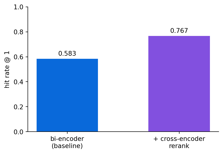
Here reranking pays off: reading each question and paragraph together, the cross-encoder pulls the right paragraph to the top far more often than the fast first pass alone, a large jump in hit rate on a corpus where the bi-encoder struggles. The latency column puts a price on that jump: the bi-encoder’s pass is a vector product over precomputed embeddings, a fraction of a millisecond, while the reranked system pays the cross-encoder’s full reading time on every query, orders of magnitude more. This row states the bargain plainly: reranking trades per-query latency you pay forever for accuracy the first pass could not reach, so it makes sense exactly where that accuracy gap exists. The same technique receives opposite verdicts on the two corpora, which is the point of the comparison. Whether reranking is worth adding cannot be settled in the abstract, because it pays exactly when retrieval is hard enough that the cheap first pass leaves room to improve. The discipline is unchanged, and it is the only thing that ports between the two cases: measure on your data, because only the numbers tell you which kind of corpus you have.
This is why the next chapter exists: our evaluations here are still crude, hit rate at 1 on a few dozen questions, and to make decisions like this with confidence we need a real evaluation toolkit: more queries, relevance judged at several ranks, the quality of generated answers as well as retrieval, and ways to grade answers that have no single right key. Chapter 9 builds this toolkit, and everything in this part has been pointing toward it.
WarningDon’t outsource this
An assistant will gladly bolt reranking, hybrid search, and contextual retrieval onto your pipeline; the code is the easy part. What it cannot do is decide whether any of them justified its cost on your data. That judgment is the whole point of this chapter, and it is the one thing you must not delegate: read the numbers, and add complexity only when they justify it.
TipCost: complexity is a cost to justify
Every technique here adds cost. Reranking is extra computation on each query. Contextual retrieval is a model call per chunk when you build the index. Query rewriting is an extra model call per question. On a system where they do not improve results, that is waste: slower answers and a larger bill for the same quality. The self-hosted reading is the same arithmetic in different units: each unnecessary step spends latency and machine capacity that could be serving other queries. Add them only when measurement shows a gap they close.
One table summarizes the chapter: what each technique fixes, where its cost falls, when it tends to pay, and what our own measurements said. The first three columns port to any retrieval system; the last one is the column you must replace with numbers from your own corpus.
| technique | failure it fixes | where the cost falls | when it pays | verdict measured here |
|---|---|---|---|---|
| reranking | the fast first pass ranks a confusable shortlist wrong | every query: cross-encoder compute and latency | corpora with many similar documents, where the shortlist is often wrong | no change on the reports corpus; a large hit-rate jump on SQuAD, paid in per-query latency |
| contextual retrieval | chunks that never name their own document | once per chunk, at indexing time | ambiguous chunks plus queries that name the document or entity | no hit-rate gain (the metric was at its ceiling), but a real, measured shift in the embedding geometry |
| hybrid search | exact terms buried by semantic matches | every query: a second index and a score blend | queries that hinge on codes, tickers, and product names | shown but never measured here; the Evaluate lab closes that gap |
| query rewriting | vague, underspecified questions | every query: one extra model call before retrieval | user-facing search where people type casually, and rewrites that keep the query’s anchors | measured on eight vague queries; in our run the rewrite drifted off-subject and hurt hit rate |
8.7 Exercises
8.7.1 Conceptual questions
Why do we use the cross-encoder only to rerank a shortlist and never to search the whole corpus?
- Its relevance scores are not comparable from one query to the next
- Reading query and chunk together is sharp but too slow for a whole corpus
- It can only score chunks that share at least one exact word with the query
- Its output is a plain score, and ChromaDB can index only vectors
Contextual retrieval prepends context to each chunk before embedding. Which failure does this fix?
- The embedding model truncates any chunk longer than its input window
- Keyword search cannot read the metadata stored alongside each chunk
- The reranker skips chunks that arrive without a document title attached
- A chunk that never names its company is hard to find with a query that does
On the report corpus, the advanced techniques did not beat plain retrieval. What is the correct lesson?
- The baseline was near the ceiling, so the extras had no gap to close
- The techniques must have been implemented wrong, since best practice says they help
- Hit rate at 1 is too coarse a metric to register any improvement at all
- Eight companies is too small a corpus for any comparison to be meaningful
A teammate proposes adding reranking, hybrid search, and query rewriting to a working RAG system all at once. What should you do first?
- Agree: the techniques are standard practice, and adding them together saves time
- Refuse all three, since this chapter showed that they do not help
- Measure the baseline, then add one technique at a time and measure each
- Swap in a different embedding model first, since that is the cheaper change
Hybrid search is most clearly worth adding when queries often hinge on:
- Long, multi-part questions that touch several topics at once
- Loose paraphrases that share no vocabulary with the documents
- Questions written in a different language than the corpus
- Exact terms such as product names, codes, or ticker symbols
On SQuAD, reranking lifted hit rate at 1 from about 0.583 to 0.767, but on the reports corpus it changed nothing. What explains the difference?
- SQuAD’s confusable paragraphs left the bi-encoder real room to improve
- The cross-encoder was trained on Wikipedia text, so SQuAD plays to its strengths
- The reports comparison scored reranking with a stricter metric than SQuAD used
- The reports comparison used cosine distance while SQuAD used the dot product
Where does the cost of contextual retrieval fall, compared with reranking?
- Both costs fall at query time, which makes both unusable at scale
- Contextual retrieval pays once per chunk at indexing; reranking pays on every query
- Contextual retrieval charges on every query; reranking is free once the model is downloaded
- Both are one-time costs paid in full when the index is first built
What does query rewriting do in a retrieval pipeline?
- It rewrites the retrieved chunks into a cleaner form for the judge to grade
- It translates the question into the language of the corpus before embedding it
- It uses a model to turn a vague question into a specific query before retrieval runs
- It fixes spelling and casing so keyword search can match exact terms
8.7.2 Build lab
Implement the full version of contextual retrieval, which upgrades the prepended context from the bare company name to a model-written sentence: use a model to write a one-sentence context for each chunk (“This passage is from Amazon’s 2023 annual report, discussing AWS segment results”), prepend that, and re-embed. Measure hit rate against the plain baseline. Report whether the richer context changed anything on this corpus, and estimate what it cost to build.
8.7.3 Evaluate lab
Construct a harder test set where you expect the baseline to struggle, with questions whose answer chunks are genuinely ambiguous about which company they describe, or that hinge on an exact figure shared across reports. Measure plain, contextual, and reranked hit rate on it. Then measure the one technique shown but never measured in this chapter, hybrid search, on the same set against the plain baseline, using BGE-M3’s sparse vectors and a 70/30 dense-sparse blend. Report which techniques, if any, justified their cost on your harder set, with the numbers that justify the claim.
NoteWhere we go next
We have leaned on a makeshift metric, hit rate at 1, three times now, and each time admitted that it was too crude to really trust. In Chapter 9 we build the evaluation toolkit that the whole book depends on: building test sets, measuring retrieval and generation properly, and using a model to judge answers that have no single correct key. After it, every later chapter measures what it builds with real instruments.