from dotenv import load_dotenv
load_dotenv()

import pandas as pd
import matplotlib.pyplot as plt9 Evaluating LLM systems
Test sets, retrieval metrics, and judging answers that have no key
A system that answers fluently can be right or wrong, and from the outside the two look the same. Telling them apart takes measurement, and so far ours has been too crude to trust: hit rate at 1 on a handful of queries, an accuracy number on thirty tickets, a keyword check on a retrieval-augmented generation (RAG) answer. This is the chapter that fixes that, and it is the most important chapter in the book. Every later chapter’s evaluation section draws on what we build here. The toolkit has two halves. When you have an answer key, you compute a metric: precision at k for retrieval, accuracy and a confusion matrix for classification. When you do not have a key, because the output is an open-ended answer or a summary with no single right form, you use a model to judge it, and then you check that the judge can be trusted. Both halves are implemented in gaba.eval.
NoteSetup for this chapter
Run in the gaba-core environment with an OPENROUTER_API_KEY. This chapter introduces gaba.eval and reuses the report corpus (Chapters 6 to 8) and the ticket data (Chapter 3). Building the corpus embeds once (the embedding model downloads on a first run); the rest is model calls.
9.1 A test set you can trust
Every metric in this chapter is computed against a test set, and a metric is only as good as the set it runs on. A test set you can trust has three properties. It is representative: the queries and documents look like what the system will really see. A common mistake is to assemble toy examples chosen to make the system look good. It is verified: a human checked the labels, because a test set with wrong answers measures nothing. And it includes the hard cases: the ambiguous tickets from Chapter 3, the queries where two answers are defensible, because a system’s behavior on the easy cases tells you almost nothing.
We already built two small test sets without calling them that: the hand-labeled ticket categories in tickets_labels.csv, and the company-tagged report corpus. We use both here. In practice, building the test set is most of the work of evaluation, and it is work you cannot skip or delegate, because every decision you make afterward rests on it.
9.2 Measuring retrieval: precision at k and MRR
Hit rate at 1 asked a single yes-or-no question: was the top result right? This discards everything about the rest of the ranking, and two better metrics preserve more of it.
Precision at k asks: of the top k results (k is a cutoff you choose, say 3 or 5), what fraction are relevant? It rewards a system that fills the top of the list with good results, which matters because a RAG system feeds several chunks to the model at once. Mean reciprocal rank (MRR) asks: how high up is the first relevant result? It rewards getting at least one good result to the very top, which matters when the model mostly needs one solid passage.
flowchart TB
    r1["rank 1: not relevant"] --> r2["rank 2: relevant"]
    r2 --> r3["rank 3: relevant"]
    r3 --> r4["rank 4: not relevant"]
    r4 --> r5["rank 5: not relevant"]
    p3["precision@3 = 2/3<br/>relevant among the top 3"] -.- r3
    rr["reciprocal rank = 1/2<br/>first relevant result is at rank 2"] -.- r2
from gaba.rag import retrieve
from gaba.eval import precision_at_k, reciprocal_rank

# A labeled query set: each query maps to the set of companies whose chunks
# count as relevant. The last query is ambiguous on purpose: a utility and a
# retailer both discuss heavy capital spending, so either company's chunks
# legitimately answer it, and the relevance set simply holds both.
queries = {
    "How many vehicles were delivered?": {"TSLA"},
    "What were the AWS cloud segment results?": {"AMZN"},
    "Tell me about turkey and packaged meat products.": {"HRL"},
    "What were the electric and gas utility operations?": {"BKH"},
    "What did the company say about capital expenditure?": {"BKH", "AMZN"},
}

rows = []
for query, companies in queries.items():
    retrieved = [hit["ticker"] for hit in retrieve(query, n=5)]
    rows.append(
        {
            "query": query[:34],
            "P@1": precision_at_k(retrieved, companies, 1),
            "P@3": precision_at_k(retrieved, companies, 3),
            "P@5": precision_at_k(retrieved, companies, 5),
            "RR": reciprocal_rank(retrieved, companies),
        }
    )

table = pd.DataFrame(rows)
table| query | P@1 | P@3 | P@5 | RR | |
|---|---|---|---|---|---|
| 0 | How many vehicles were delivered? | 1.0 | 0.666667 | 0.4 | 1.00 |
| 1 | What were the AWS cloud segment re | 1.0 | 1.000000 | 1.0 | 1.00 |
| 2 | Tell me about turkey and packaged | 1.0 | 1.000000 | 1.0 | 1.00 |
| 3 | What were the electric and gas uti | 1.0 | 1.000000 | 1.0 | 1.00 |
| 4 | What did the company say about cap | 0.0 | 0.000000 | 0.4 | 0.25 |
print(f"mean P@3: {table['P@3'].mean():.2f}")
print(f"MRR:      {table['RR'].mean():.2f}")
mean P@3: 0.73
MRR: 0.85Now the numbers carry structure: mean precision at 3 tells us how clean the top of the ranking is across queries, while MRR tells us how reliably a relevant chunk reaches the top. These are the numbers you track when you change a retrieval component, the baseline that Chapter 8’s techniques would have to beat to justify their cost. The capital-expenditure row shows how ambiguity is handled. A common mistake is to drop such a query because no single company is “the” answer; here the relevance set simply holds two companies, and the metrics need no modification because they were defined against a set from the start. Multi-item relevance sets are the normal case on real corpora, where several documents can legitimately answer one query, and an evaluation that keeps only single-answer queries quietly selects for the easy ones. One caveat about this corpus: we are treating “relevant” as “from the correct company,” a coarse proxy, so precision at k here measures company-purity, leaving unmeasured whether each passage truly answers the question. A chunk of boilerplate from the right company counts as relevant. On real data you judge relevance at the passage level, which makes the metric sharper, because precision at k is only ever as good as the relevance judgments behind it.
9.3 Measuring classification: the confusion matrix
When the task is classification, accuracy is the summary figure, but the confusion matrix supplies the detail. Beyond how often the system is wrong, it shows which categories it mistakes for which, which is what tells you whether an error is a genuine mistake or a defensible disagreement. We run the Chapter 3 triage over all thirty labeled tickets and build one.
TipWith an AI coding tool
Wiring the ThreadPoolExecutor around triage, matching predictions back to their ticket ids, and building the crosstab into a confusion matrix is exactly the kind of harness code worth handing to an assistant, because it is bookkeeping that requires no judgment. What you must still decide yourself is which off-diagonal cells are worth investigating and whether a given miss names a real model error or a debatable label of your own. Let the tool draft the loop; keep the reading of the matrix for yourself.
from enum import Enum
from typing import Literal
from pydantic import BaseModel
from concurrent.futures import ThreadPoolExecutor
from gaba.llm import call_structured
from gaba.data import load_tickets, load_ticket_labels, TICKET_CATEGORIES

TicketCategory = Enum("TicketCategory", {c: c for c in TICKET_CATEGORIES}, type=str)

class Triage(BaseModel):
    category: TicketCategory

tickets = load_tickets()  # all 30, for a matrix with enough cells to read
gold = dict(zip(load_ticket_labels()["ticket_id"], load_ticket_labels()["category"]))

def triage(text: str) -> str:
    result = call_structured(text, Triage,
                             system="Classify the support ticket into one category.")
    return result.data.category.value

with ThreadPoolExecutor(max_workers=8) as pool:
    pred = list(pool.map(triage, tickets["text"]))
true = [gold[t] for t in tickets["ticket_id"]]

confusion = pd.crosstab(
    pd.Series(true, name="actual"), pd.Series(pred, name="predicted")
)
accuracy = sum(p == t for p, t in zip(pred, true)) / len(pred)
print(f"accuracy on {len(pred)} tickets: {accuracy:.0%}")
accuracy on 30 tickets: 100%The matrix is easiest to scan as a heatmap, where any off-diagonal count stands out at a glance.
fig, ax = plt.subplots(figsize=(6, 5))
im = ax.imshow(confusion.values, cmap="Blues")
ax.set_xticks(range(len(confusion.columns)), confusion.columns,
              rotation=45, ha="right")
ax.set_yticks(range(len(confusion.index)), confusion.index)
ax.set_xlabel("predicted")
ax.set_ylabel("actual")
for i in range(confusion.shape[0]):
    for j in range(confusion.shape[1]):
        count = confusion.values[i, j]
        ax.text(j, i, str(count), ha="center", va="center",
                color="white" if count > confusion.values.max() / 2 else "black")
plt.tight_layout()
plt.show()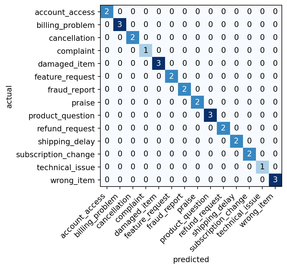
A perfectly diagonal matrix means every prediction matched its label. Any off-diagonal cell names a specific confusion, “we called a cancellation a subscription change,” and that name is an instruction: pull the ticket behind the cell and read it against both categories. With all thirty tickets in the matrix, the off-diagonal counts that appear are exactly where to spend that minute, because each one resolves into one of two findings. Sometimes the model is simply wrong, and the cell names the category boundary it cannot distinguish. And sometimes you reread the ticket and find your own label was the debatable one, a complaint that really is mostly a refund request, which Chapter 3 warned these tickets contain by design. The second finding is just as valuable as the first: it means the matrix is a check on the test set as well as on the model, and a label you revise after this kind of rereading makes every later measurement against it sharper.
9.4 Measuring abstention: two numbers for two jobs
Chapter 7 demonstrated that our RAG system refuses questions its documents cannot answer, and promised that this chapter would measure that behavior, which so far we have only trusted. A RAG system has two jobs, answering what it can and declining what it cannot, and a single score merges the tradeoff between them into one number: a system that answers everything succeeds at the first job by failing the second, and a system that refuses everything does the reverse. So we score the two jobs separately, on a small set of answerable and unanswerable questions, and report two numbers.
from gaba.rag import rag_answer

REFUSAL = ["cannot find", "could not find", "not in the", "unable", "does not",
           "not contain", "no information", "not available"]

answerable = {
    "Which business segments does Amazon report results for?": ["aws"],
    "What kind of utility business does Black Hills operate?": ["electric", "gas"],
    "What kinds of products does Hormel make?": ["meat", "turkey", "food", "pork", "spam"],
}
unanswerable = [  # plausibly in-domain, but absent from the 2023 reports
    "What was Amazon's total advertising revenue in 2019?",
    "How many vehicles did Tesla deliver in 2015?",
]

answered = sum(any(e in rag_answer(q)[0].lower() for e in expected)
               for q, expected in answerable.items())
abstained = sum(any(r in rag_answer(q)[0].lower() for r in REFUSAL)
                for q in unanswerable)
print(f"answer rate when answerable:    {answered}/{len(answerable)}")
print(f"abstain rate when unanswerable: {abstained}/{len(unanswerable)}")
answer rate when answerable: 3/3
abstain rate when unanswerable: 2/2Both numbers matter, and they pull against each other: a stricter system prompt pushes the abstain rate up and risks dragging the answer rate down, so any change to the grounding instructions should be checked against both. The refusal check here is still a crude keyword match, and the next section builds the tool that replaces it: a judge that can grade whether an answer is actually grounded in its sources, refusals included. The set is also tiny, five questions, so treat the numbers as a smoke test; the practice scales by adding cases, especially unanswerable ones that sound answerable, which Chapter 7 showed are the cases that matter.
9.5 Judging answers without a key: the LLM as judge
Retrieval and classification have answer keys. A generated answer usually does not: there are many good ways to answer “how did Amazon Web Services (AWS) do this year,” and no single string to match against. What we can check, however, is whether the answer is faithful to its source and relevant to the question. For this, we use a large language model (LLM) as a judge, prompted to grade strictly against the provided context. The judge returns a third verdict as well: whether the answer is complete. We use this in Chapter 10 when a question requires several facts and a fluent answer can easily omit one. We run this with llm_judge, the gaba function that takes a question, an answer, and the source context, returning those three verdicts (faithful, relevant, and complete).
flowchart LR
    q["Question"] --> judge["Judge model<br/>with a rubric"]
    a["System answer"] --> judge
    ctx["Source context"] --> judge
    judge --> v["Verdict:<br/>faithful? relevant?"]
    v --> agg["Aggregated scores<br/>over a sample"]
    pin["The judge is itself a model:<br/>pin its version and prompt"] -.- judge
from gaba.eval import llm_judge

context = "[AMZN] AWS segment sales grew 13% year over year to $90.8 billion in 2023."
question = "How fast did AWS grow in 2023?"

answers = {
    "faithful": "AWS grew 13% year over year in 2023, reaching $90.8 billion.",
    "hallucinated": "AWS grew 45% in 2023, its fastest year ever, reaching $200 billion.",
    "off-topic": "Amazon was founded in 1994 by Jeff Bezos.",
}

for label, answer in answers.items():
    verdict = llm_judge(question, answer, context)
    print(f"{label:13s} faithful={verdict.faithful!s:5s} relevant={verdict.relevant!s:5s}")
faithful faithful=True relevant=True
hallucinated faithful=False relevant=True
off-topic faithful=False relevant=FalseThe judge marks the faithful answer faithful, catches the hallucinated one (the 45 percent and the $200 billion are nowhere in the context), and flags the off-topic answer as neither faithful nor relevant. One detail in the hallucinated row deserves attention: the judge also marked it not relevant, even though an answer with wrong numbers about AWS growth plainly addresses the question; the judge let correctness influence a dimension that was supposed to be about topic, a small live example of the judge biases we return to below. This is how you evaluate a RAG system’s answers, which the retrieval metrics leave unexamined: run the judge over a sample of real questions and track the faithfulness rate. A system whose retrieval is perfect but whose answers are not grounded in the sources is still broken, and only judging the answers reveals it.
9.6 Validating the judge against human labels
A judge is itself a model, and a model can be wrong, so the judge needs evaluating too. The remedy is to check it against human labels: take a set of answers a person has graded, have the judge grade them, and measure how often they agree.
Metric: agreement between the judge and human labels on faithfulness.
Test set: twelve answers a human has labeled faithful or not, four of them engineered to sit on the boundary where humans themselves hesitate.
Baseline: a judge guessing at random would land near chance, roughly half on a balanced set, so anything well above that is signal.
# Twelve answers, each with a human's faithfulness label. The first eight are
# clear-cut. The last four are engineered borderline cases, one per failure
# family, and on each a careful human could defend either label; the label
# below is OUR ruling, stated definitely so the judge has something to
# disagree with:
#   - characterization: "modest" and "a slowdown" are claims the context
#     neither states nor contradicts. We rule strictly: not faithful.
#   - derived figure: 13% growth to $90.8B implies roughly $10B of growth,
#     computable from the context but never stated. We rule: faithful.
#   - rounding: "about one-eighth" restates 13%. We rule: faithful.
#   - faithful but incomplete: supported, and silent on every figure.
#     We rule: faithful (incompleteness is a different dimension).
labeled = [
    ("AWS grew 13% in 2023.", True),
    ("AWS grew about 13% year over year.", True),
    ("AWS revenue reached $90.8 billion.", True),
    ("AWS sales were $90.8 billion, up 13% from the prior year.", True),
    ("AWS grew 30% in 2023.", False),
    ("AWS shrank in 2023.", False),
    ("AWS reached $500 billion in 2023.", False),
    ("AWS was Amazon's fastest-growing segment in 2023.", False),
    # The engineered borderline cases:
    ("AWS posted modest growth of 13%, a slowdown for the segment.", False),
    ("AWS grew by roughly $10 billion in 2023.", True),
    ("AWS grew by about one-eighth in 2023.", True),
    ("AWS segment sales increased in 2023.", True),
]

with ThreadPoolExecutor(max_workers=8) as pool:
    verdicts = list(pool.map(lambda case: llm_judge(question, case[0], context),
                             labeled))

agree, disagreements = 0, []
for (answer, human_faithful), verdict in zip(labeled, verdicts):
    if verdict.faithful == human_faithful:
        agree += 1
    else:
        disagreements.append((answer, human_faithful, verdict))

print(f"judge agreement with human labels: {agree}/{len(labeled)}")
judge agreement with human labels: 11/12A score short of perfect is not a verdict by itself; the chapter’s own rule is to read the results, so we look at exactly where the judge and the human parted ways.
if not disagreements:
    print("no disagreements on this run")
for answer, human_faithful, verdict in disagreements:
    print(f"human said faithful={human_faithful}, judge said {verdict.faithful}")
    print(f"  answer:    {answer}")
    print(f"  reasoning: {verdict.reasoning}")
human said faithful=False, judge said True
answer: AWS posted modest growth of 13%, a slowdown for the segment.
reasoning: The answer is faithful and relevant, but it does not provide the total sales figure for AWS in 2023, which was explicitly asked for in the question.The list of disagreements is more informative than the score, and the disagreements, when they appear, should fall on the four engineered cases at the end, while the judge and the human agree on the clear-cut eight. Each of the four probes a different boundary, and each boundary has a defensible position on both sides. The characterization case asks whether words like “modest” and “a slowdown” need their own support or ride along free with the correct number; we ruled strictly, so a lenient judge that waves them through parts ways with us, and a strict one agrees. The derived figure asks whether the judge will credit arithmetic the context licenses but never states; a judge that refuses is merely strict. The rounding case asks whether “about one-eighth” is 13 percent. And the incomplete answer separates faithfulness from completeness: every word of it is supported, it just answers less than was asked, and a judge that marks it unfaithful is grading the wrong dimension, the one rubric confusion the set is built to expose. Whichever way each verdict falls in your run, the reading is the same. When judge and human part ways on a case the humans themselves found contestable, the disagreement measures the ambiguity of the case, whereas a defect in the judge would surface on the clear-cut cases, and the fix is a sharper rubric, one that says explicitly how to treat characterization, derivation, and rounding. A miss on a clear-cut case would be the alarming kind; misses on the engineered four mean the test set is working as designed. And a perfect score on this set proves less than it seems: it mostly says our rulings and this judge’s leanings happen to line up today, which is worth knowing and worth re-checking whenever the judge model or the rubric changes. An agreement rate read together with where the misses fall is worth more than a clean sweep on a test set with no hard cases, because a set where everything sits at the ceiling has not tested the judge at all.
When the judge agrees with human labels often, and the disagreements land where your own labels were weakest, you can use it at scale with some confidence; when it does not, the judge needs a better prompt or a stronger model before you trust its verdicts. This check is not optional: a judge you have never validated is just another unmeasured system, and the whole point of this chapter is to stop putting unmeasured systems into use. Three cautions worth carrying forward: judges have biases (the literature reports they tend to favor longer answers and the first option in a pairwise comparison, though your own judge may lean either way, which is why you measure), so design around them; pin the judge’s model and prompt, because changing either silently changes your metric; and in production, judge a sample, because judging every call has a real cost.
9.7 Pairwise judging and position bias
The judge so far grades one answer on an absolute rubric. The other judging mode is pairwise: show the judge two candidate answers and ask which is better. This is how you compare two prompts, two models, or two retrieval settings head to head. Pairwise verdicts feel more decisive than absolute grades, which is why the two biases above, so far only mentioned, need to be measured. We can measure both with one experiment. Build pairs where both answers carry the same context-supported facts and differ only in length, so the only correct verdict is indifference, then judge every pair twice, once in each order.
from pydantic import Field

class PairwiseVerdict(BaseModel):
    winner: Literal["A", "B"] = Field(description="the better answer")
    reasoning: str = Field(description="one sentence explaining the choice")

def pairwise_judge(question: str, answer_a: str,
                   answer_b: str, context: str) -> PairwiseVerdict:
    prompt = (f"Question: {question}\n\nContext:\n{context}\n\n"
              f"Answer A:\n{answer_a}\n\nAnswer B:\n{answer_b}\n\n"
              "Which answer is better?")
    return call_structured(
        prompt, PairwiseVerdict,
        system="You compare two answers to the same question against the "
               "provided context and pick the better one.",
    ).data

# Eight short answers, all fully supported by the context. Each is paired with
# a padded twin that adds words but no facts, so within every pair the two
# answers are equally faithful and any systematic preference is bias.
facts = [
    "AWS grew 13% in 2023.",
    "AWS sales reached $90.8 billion in 2023.",
    "AWS grew 13%, reaching $90.8 billion.",
    "AWS sales were $90.8 billion, up 13%.",
    "In 2023 AWS grew 13% year over year.",
    "AWS ended 2023 at $90.8 billion in sales.",
    "Year-over-year growth for AWS was 13%.",
    "AWS posted 13% growth and $90.8 billion in sales.",
]
PAD = ("To answer the question directly, and summarizing only what the "
       "provided context supports: ")
pairs = [(f, PAD + f + " That is the figure the context reports for the "
          "AWS segment in 2023.") for f in facts]

def judge_both_orders(pair):
    short, long = pair
    first = pairwise_judge(question, short, long, context)   # long sits at B
    second = pairwise_judge(question, long, short, context)  # long sits at A
    long_wins = (first.winner == "B") + (second.winner == "A")
    # If the judge names the same letter in both orders, the letter pointed at
    # a different answer each time: the verdict followed the seat alone.
    flipped = first.winner == second.winner
    return long_wins, flipped

with ThreadPoolExecutor(max_workers=8) as pool:
    outcomes = list(pool.map(judge_both_orders, pairs))

print(f"long answer preferred: {sum(o[0] for o in outcomes)}/{2 * len(pairs)} verdicts")
print(f"verdict flipped with order: {sum(o[1] for o in outcomes)}/{len(pairs)} pairs")
long answer preferred: 0/16 verdicts
verdict flipped with order: 0/8 pairsThe two numbers should be read against what the pairs were built to be: equal. Any consistent lean in the first line, in either direction, is presentation bias, a verdict that tracks style alone, because the padded twin asserts nothing its short partner does not. The lean documented across the literature runs toward longer answers; in our run this judge leaned hard the other way, punishing the padding nearly every time, and this inversion is itself the lesson. The folklore describes judges in general; your judge, with your rubric and your prompt, has its own lean, and the only way to learn its direction is to measure it on pairs whose right answer you know, here “indifference.” The second line is the deeper warning: every flipped pair is a verdict that changed when A and B swapped seats, a judgment that belonged to the seating order alone. The mitigations are mechanical once you know to apply them: randomize which answer takes which position, judge each pair in both orders, keep only the verdicts that agree across orders, and score the rest as ties. This costs twice the judge calls per comparison; de-biasing a measurement usually means doing more measuring.
Everything this chapter has said about operating a judge fits in four rows, and each row exists because of what goes wrong without it.
| practice | why | what breaks if you skip it |
|---|---|---|
| validate against human labels | the judge is a model and can be wrong | you scale verdicts you never checked, and every downstream number inherits their unknown error rate |
| pin the judge’s model and prompt | a metric must mean the same thing across runs | a silent model upgrade moves your scores, and you read the drift as a real regression |
| design around known biases | judges favor longer answers and the first position | verbose answers win your comparisons, and pairwise verdicts depend on presentation order |
| judge a sample in production | every judgment is a model call with real cost | the evaluation bill grows with traffic until it rivals the serving bill |
TipCost: evaluation is a model call too
An LLM judge is a model call per item judged, so evaluating a thousand answers costs about what generating a thousand answers costs. Therefore, in production, you judge only a representative sample of requests. Self-hosted, the same arithmetic appears as throughput: every judged answer occupies capacity that could be serving traffic, which is one more reason to sample. The answer-key metrics, precision at k, accuracy, are worth using wherever you have a key, because they are free to compute. Spend the judge where there is no key, and spend it on a sample.
WarningDon’t outsource this
You can let an assistant write the evaluation loop, the metric functions, and the confusion-matrix code. You cannot let it build your test set or read your results. Choosing representative cases, verifying labels, and deciding whether a faithfulness rate is good enough for your stakes are the judgments the whole exercise exists to support, and they are yours.
9.8 Exercises
9.8.1 Conceptual questions
A system scores perfectly on hit rate at 1 but poorly on precision at 3. What is happening?
- The top result is right while the next results are irrelevant
- The first relevant result is buried below rank three in the list
- The test set contains queries with no relevant chunks at all
- The ranking is fine but the relevance labels behind it are wrong
Which property does the chapter require of a test set you can trust?
- Labels produced by the model under test, so the formats agree
- Only clear-cut cases, so that every label is beyond dispute
- Verified labels, because a set with wrong answers measures nothing
- The largest possible size, even if the labels go unchecked
A query’s first relevant result appears at rank 4. Its reciprocal rank is:
- 0.4
- 0.25
- 4.0
- 0.75
What does a confusion matrix show that a single accuracy number does not?
- The cost and latency of every prediction next to its label
- How confident the model was about each individual prediction
- How the accuracy figure changes as the test set grows larger
- Which categories the system mistakes for which other ones
Why do we grade RAG answers with an LLM judge, when we could match them against a correct answer string?
- A judge costs less to run than the answer-key metrics do
- Using a judge removes the need to build and verify a test set
- An open-ended answer has many valid forms and no single string to match
- A judge model grades more consistently than human labelers can
Before trusting an LLM judge at scale, the chapter says to:
- Measure its agreement with human labels on a graded sample
- Switch to the largest available model, which removes the need to check
- Run it twice on every answer and keep only the matching verdicts
- Set its temperature to zero so its verdicts become deterministic
Which of these is a documented bias of LLM judges?
- Marking short answers unfaithful no matter how accurate they are
- Refusing to grade any answer that quotes figures from the context
- Growing harsher as the source context they must read gets longer
- Favoring longer answers and the first option when comparing pairs
On the report corpus, “relevant” was defined as “from the correct company.” What does that make the precision figures?
- Exact, because the company labels come from metadata a human verified
- Company-purity scores: any chunk from the right company counts as relevant
- Understated, because the ticker metadata is missing from many of the chunks
- Incomparable across queries that target different companies
9.8.2 Build lab
Extend the retrieval evaluation to compute recall at k as well as precision at k, using gaba.eval.recall_at_k. Add three new labeled queries. Report which metric moved most when you increased k from 3 to 5, and explain in one sentence what that tells you about the ranking.
9.8.3 Evaluate lab
This exercise is open-ended. Take ten real RAG answers from Chapter 7’s system (or generate them), hand-label each as faithful or not, then run llm_judge over them and measure agreement. Report the agreement rate and, for every case where the judge disagreed with you, decide who was right. Then state whether you would trust this judge to grade a thousand answers unattended, and defend the call with your number.
NoteWhere we go next
We can now measure what we build, which means the rest of the book can make claims and back them with numbers. Chapter 10 uses that ability immediately. It is about context engineering: how to decide what goes into a model’s limited context window, and how to tell, by measuring, whether stuffing in more actually helps or quietly hurts.