flowchart LR
    img["Image<br/>(chart, scanned page,<br/>shelf photo, video frame)"] --> vlm["Vision-language<br/>model"]
    q["Text question"] --> vlm
    vlm --> ans["Answer grounded in<br/>what the image shows"]
    ans --> exact["Text and labels:<br/>read near-exactly"]
    ans --> est["Unlabeled quantities:<br/>estimates only"]
19 Vision-language models for documents, scenes, and video
Reading charts, invoices, shelves, and camera footage
Not all business data is text. A great deal of it is captured in scanned invoices, photographed receipts, charts buried in a slide deck, retail shelves, and the footage from the security camera over the checkout. A vision-language model reads images the way a language model reads text: you send it a picture and a question, and it answers.
In this chapter, we work through the ladder of vision tasks an analyst actually meets: reading a chart, extracting a document with checkable arithmetic, auditing a scene with questions and counts, and turning video into a time series by sampling frames. Throughout the chapter we draw a careful line between what these models read reliably, the text and labels in an image, and what they only estimate or count by eye.
NoteIn the running system
Some of what our desk handles is not text at all, such as a scanned invoice or a chart in a slide. This chapter gives the system eyes, reading documents and scenes into the same structured outputs the rest of the pipeline consumes.
The chapter climbs this ladder one task at a time, and the rungs differ in what the model actually reads and in what you get for free to check it against:
| Task | What is actually read | Reliability | Free validation |
|---|---|---|---|
| Chart | axis text and data labels; bar heights only by eye | near-exact for labels, estimate for unlabeled quantities | render the same chart with labels, or compare to source data |
| Document (invoice, form) | printed fields and amounts | near-exact | internal arithmetic: line items must sum to the totals |
| Scene (shelf, dock) | product labels read well; counts located by eye | labels solid, counting wobbles | repeat the audit and watch which fields hold still |
| Video (camera feed) | one sampled frame at a time, plus its timestamp | per-frame, same as scenes | consistency across adjacent frames; scripted test clips |
NoteSetup for this chapter
Run in the gaba-core environment with an OPENROUTER_API_KEY. This chapter introduces gaba.llm.call_vision and uses the book’s default model, which is multimodal (it accepts images as well as text). Every image and the video clip are included with the book (assets/data/images/, assets/data/video/). The invoice is drawn by scripts/make_vision_assets.py with its values known by construction; the shelves and the checkout clip are AI-generated imagery whose contents we counted by hand and committed as gold labels (the clip is provided both as a GIF for the page and as checkout.mp4 for the native-video call). Either way each reading can be checked against known values, and your own photos, scans, and camera feeds work in the same calls.
from dotenv import load_dotenv

def _pil_bytes(im):
    import io as __io
    b = __io.BytesIO(); im.save(b, format="PNG"); return b.getvalue()
load_dotenv()

import io
import matplotlib.pyplot as plt
19.1 Tools in this chapter
| Tool | Why we use it here | Alternatives | Trade-off |
|---|---|---|---|
| The book’s default multimodal model | reads an image and a question together and returns text or structured data, through the same API as every other chapter | open vision-language models (Qwen-VL, InternVL); other hosted models (Gemini) | one call with no setup against estimating unlabeled quantities only by eye |
The tooling-landscape appendix lists the current options for each.
19.2 Reading an image
Sending an image uses the familiar chat call, with the image attached to the message, and gaba.llm.call_vision handles the encoding. We begin with a chart that has no data labels, only bars, and ask the model to read the values. The companies and their revenues are invented, which matters more than it may seem: real company revenues are all over the model’s training data, so a chart of Amazon and Tesla could be “read” from memory, with the pixels never consulted. With fictional firms, whatever the model reports, it read from the image.
from gaba.llm import call_vision

companies = ["Northwind", "Cascadia", "Bluepeak", "Harborlight"]
revenues = [412.0, 87.0, 9.0, 3.0]

def revenue_chart(with_labels: bool) -> bytes:
    fig, ax = plt.subplots(figsize=(7, 4.5))
    bars = ax.bar(companies, revenues, color="steelblue")
    ax.set_ylabel("annual revenue (billions USD)")
    ax.set_title("Company revenue")
    if with_labels:
        for bar, value in zip(bars, revenues):
            ax.text(bar.get_x() + bar.get_width() / 2, value, f"{value}",
                    ha="center", va="bottom")
    buf = io.BytesIO(); fig.savefig(buf, format="png", dpi=150); plt.close(fig)
    return buf.getvalue()

from IPython.display import Image, display

unlabeled = revenue_chart(with_labels=False)
display(Image(unlabeled))  # this is the image the model will read

result = call_vision("Read this bar chart. For each company, give its revenue value.",
                     unlabeled)
print(result.text)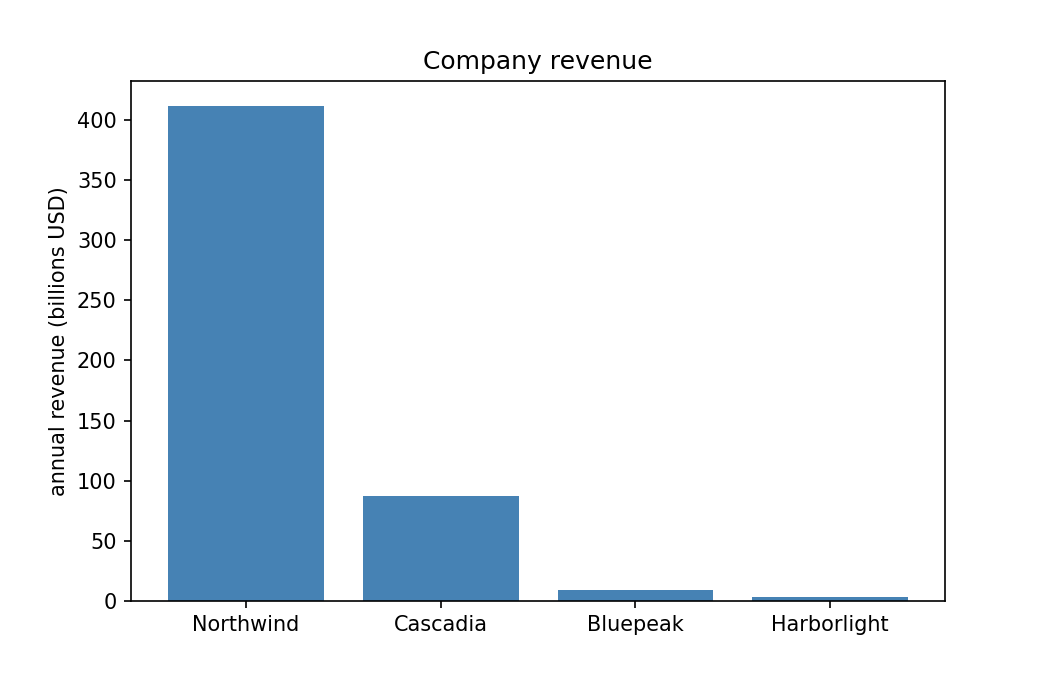
Here are the revenue values for each company, as read from the bar chart:

* **Northwind:** 410 billion USD
* **Cascadia:** 85 billion USD
* **Bluepeak:** 10 billion USD
* **Harborlight:** 5 billion USD
The model identifies every company and reads the chart, but its numbers are estimates: it gauged each bar’s height against the axis, much as you would at a glance, and rounded. The tall Northwind bar is easy to place; the short Bluepeak and Harborlight bars, a few pixels high against a 400-billion axis, are much harder. Because it cannot measure pixels, an unlabeled bar yields only an approximate value. This is the boundary that matters: a vision model understands what an image shows, but it reads unlabeled quantities by eye.
19.3 Text in images is read nearly exactly
The picture changes when the value is written on the image as text. Vision models read text in an image accurately, which is why scanned documents, labeled charts, and forms are where they excel. The same chart with data labels yields near-exact figures.
labeled = revenue_chart(with_labels=True)
display(Image(labeled))

result = call_vision(
    "Read the labeled values from this chart. Return one line per company as "
    "'Company: value'.",
    labeled)
print(result.text)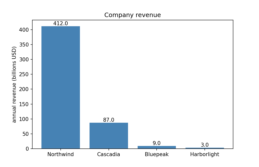
Northwind: 412.0
Cascadia: 87.0
Bluepeak: 9.0
Harborlight: 3.0
Now the figures are near-exact, because the model reads the value as printed text, which requires no estimate of a bar’s height. Even reading is not infallible, so verify extractions against values you can check whenever the document offers any, a printed total, a row count, a checksum. This is the practical rule for using vision on business documents: use it to read what is written, the line items on an invoice, the total on a receipt, the labels on a chart, and be cautious when you ask it to estimate something the image only depicts.
19.4 Reading a document: an invoice that checks itself
Charts were the warm-up; the workhorse case is documents. We read a synthetic invoice whose true values we control, and extract it into the structured form Chapter 3 taught, by the same two-step pattern as above: the vision model reads, call_structured parses.
from gaba import DATA_DIR

invoice_png = (DATA_DIR / "images" / "invoice.png").read_bytes()
display(Image(invoice_png, width=560))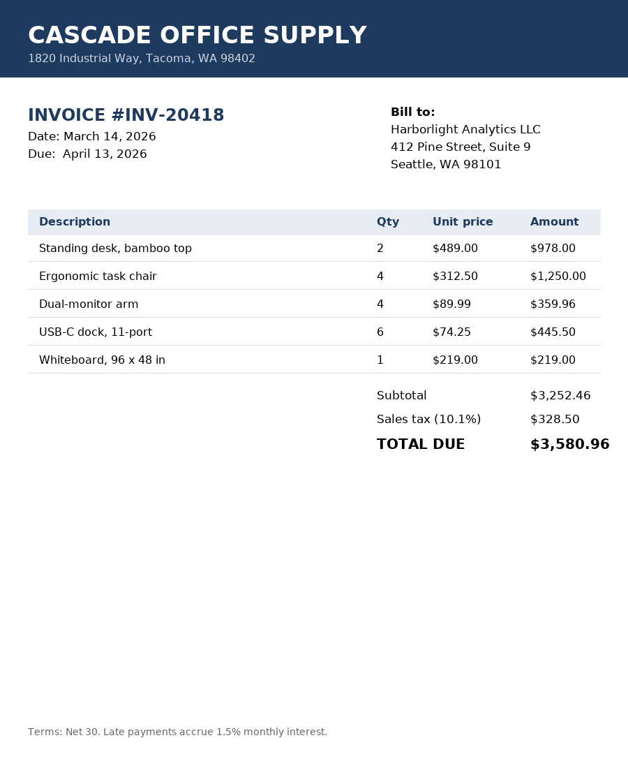
from pydantic import BaseModel
from gaba.llm import call_structured

class InvoiceFacts(BaseModel):
    invoice_number: str
    vendor: str
    line_item_count: int
    subtotal: float
    tax: float
    total: float

reply = call_vision(
    "Read this invoice. Report the invoice number, vendor, number of line "
    "items, subtotal, tax, and total due.",
    invoice_png, max_tokens=400).text
inv = call_structured("Extract the invoice fields from this text:\n" + reply,
                      InvoiceFacts).data
print(inv)
invoice_number='INV-20418' vendor='CASCADE OFFICE SUPPLY' line_item_count=5 subtotal=3252.46 tax=328.5 total=3580.96A document is better than a chart in one important way: it carries its own arithmetic. The line amounts must sum to the subtotal, and subtotal plus tax must equal the total, so the extraction can be checked for internal consistency before anyone compares it to a source system. This is the cheapest validation in the book, and real invoices offer it for free.
import json

consistent = abs((inv.subtotal + inv.tax) - inv.total) < 0.01
gold = json.loads((DATA_DIR / "images" / "vision_gold.json").read_text())["invoice"]
pairs = [("invoice_number", "invoice_number"), ("line_item_count", "line_items"),
         ("subtotal", "subtotal"), ("tax", "tax"), ("total", "total")]
exact = sum(getattr(inv, field) == gold[key] for field, key in pairs)
print(f"arithmetic consistent: {consistent} | fields exactly right: {exact}/5")
arithmetic consistent: True | fields exactly right: 5/5Both checks matter, and they catch different failures: the gold comparison needs ground truth we normally do not have, while the arithmetic check works on any invoice. An extraction that fails the arithmetic check goes to a person, no gold labels required, which is the abstention pattern from Chapter 7, applied to accounts payable.
Our invoice is a crisp render; real ones arrive as photocopies and phone photos. How good does the scan have to be? Re-running the same extraction on degraded copies turns that question into a measurement.
TipWith an AI coding tool
Turning the one-off invoice call into a reusable extract_invoice function, and writing a degraded helper that composes a resize and a Gaussian blur, is routine refactoring an assistant drafts well. Ask for it, then check the part that matters: that degraded is a pure function of its inputs so the sweep below compares scan quality and nothing else, and that extract_invoice still returns the same InvoiceFacts structure at every degradation level, so a silent parse error cannot be mistaken for a genuinely bad read.
from PIL import Image as PILImage, ImageFilter
import pandas as pd

base_img = PILImage.open(DATA_DIR / "images" / "invoice.png")

def degraded(scale: float = 1.0, blur: float = 0.0) -> bytes:
    img = base_img
    if scale < 1.0:
        w, h = img.size
        img = img.resize((int(w * scale), int(h * scale)), PILImage.LANCZOS)
    if blur:
        img = img.filter(ImageFilter.GaussianBlur(blur))
    buf = io.BytesIO(); img.save(buf, format="PNG"); return buf.getvalue()

def extract_invoice(png: bytes) -> InvoiceFacts:
    text = call_vision(
        "Read this invoice. Report the invoice number, vendor, number of line "
        "items, subtotal, tax, and total due.", png, max_tokens=400).text
    return call_structured("Extract the invoice fields from this text:\n" + text,
                           InvoiceFacts).data

levels = [("100%", dict()), ("75%", dict(scale=0.75)), ("50%", dict(scale=0.50)),
          ("33%", dict(scale=0.33)), ("100% + blur", dict(blur=2.0))]
rows = []
for name, kwargs in levels:
    e = extract_invoice(degraded(**kwargs))
    exact = sum(getattr(e, field) == gold[key] for field, key in pairs)
    rows.append({"quality": name, "fields exact": f"{exact}/5",
                 "arithmetic consistent": abs((e.subtotal + e.tax) - e.total) < 0.01})
pd.DataFrame(rows)| quality | fields exact | arithmetic consistent | |
|---|---|---|---|
| 0 | 100% | 5/5 | True |
| 1 | 75% | 5/5 | True |
| 2 | 50% | 5/5 | True |
| 3 | 33% | 5/5 | True |
| 4 | 100% + blur | 5/5 | True |
Wherever the fields fall off in this table is the cliff, and it belongs to this layout, this font size, and this model: a measured minimum scan quality, which without the sweep we could only have guessed. Watch the arithmetic column on the way down, too. A misread digit rarely stays consistent with the printed totals, so when degradation starts corrupting fields, the consistency check tends to trip alongside them, which is what makes it a useful tripwire on documents you have no gold for. The same few-call sweep, run on a sample of your own scans, tells you whether the photos coming in from the field sit above your cliff or below it, before the pipeline silently accepts them.
19.5 Asking questions about a scene: the shelf audit
Documents are mostly reading. Scenes, a shelf, a loading dock, a factory station, add two harder skills: answering open questions about what is depicted, and counting. To illustrate, we audit a photorealistic AI-generated retail shelf whose contents we counted by hand: how many facings of each product, how many slots are tagged out of stock, whether anything is misplaced. Generated imagery with hand-labeled gold gives us the same checkability as the invoice; a phone photo of a real aisle drops into the identical call.
shelf_png = (DATA_DIR / "images" / "shelf_clean.png").read_bytes()
display(Image(shelf_png, width=640))

for q in ["What products are on this shelf?",
          "Are any slots empty or out of stock?",
          "Is any product on the wrong shelf?"]:
    answer = call_vision(q, shelf_png, max_tokens=120).text.strip()
    print(f"Q: {q}\nA: {answer}\n")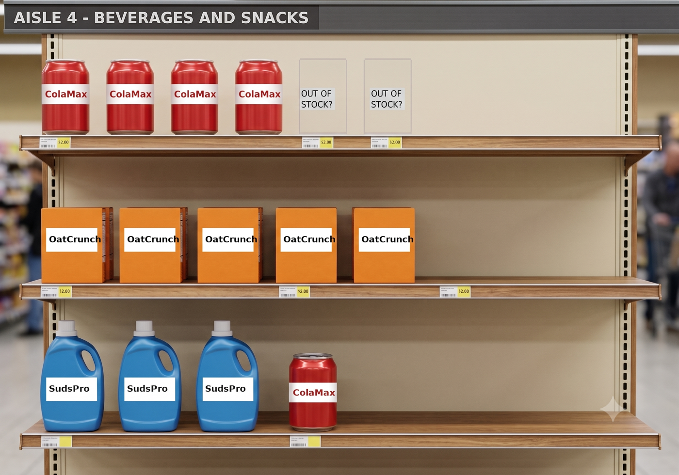
Q: What products are on this shelf?
A: On the top shelf, there are four cans of "ColaMax". Next to these are two empty spots labeled "OUT OF STOCK?".

On the middle shelf, there are four boxes of "OatCrunch".

On the bottom shelf, there are three blue jugs labeled "SudsPro" and one red can labeled "ColaMax".

Q: Are any slots empty or out of stock?
A: Yes, there are slots that are empty or out of stock.

On the top shelf, there are two slots labeled "OUT OF STOCK?".

On the second shelf, there are empty slots to the right of the "OatCrunch" boxes.

On the bottom shelf, there is an empty slot to the right of the "ColaMax" can.

Q: Is any product on the wrong shelf?
A: The **ColaMax** can on the bottom shelf appears to be on the wrong shelf. Aisle 4 is labeled as "Beverages and Snacks," and while the other ColaMax cans are on the top shelf as part of a beverage display, this solitary can is on the bottom shelf alongside cleaning supplies ("SudsPro").
Open questions give a feel for what the model sees, but an audit needs numbers. The same image, extracted into a structured count and scored against what we drew:
class ShelfAudit(BaseModel):
    colamax_count: int
    oatcrunch_count: int
    sudspro_count: int
    out_of_stock_tags: int
    misplaced_item_present: bool

AUDIT_PROMPT = (
    "Audit this shelf. Count the total ColaMax containers anywhere in the "
    "image, the OatCrunch boxes, the SudsPro containers, and the slots "
    "marked OUT OF STOCK. Say whether any product sits on the wrong shelf.")

reply = call_vision(AUDIT_PROMPT, shelf_png, max_tokens=300).text
audit = call_structured("Extract the audit from this text:\n" + reply,
                        ShelfAudit).data
g = json.loads((DATA_DIR / "images" / "vision_gold.json").read_text())["shelf_clean"]
checks = {
    "colamax (5, incl. misplaced)": audit.colamax_count == g["colamax_total"],
    "oatcrunch (5)": audit.oatcrunch_count == g["oatcrunch"],
    "sudspro (3)": audit.sudspro_count == g["sudspro"],
    "out-of-stock tags (2)": audit.out_of_stock_tags == g["out_of_stock_tags"],
    "misplaced flagged": audit.misplaced_item_present,
}
for name, ok in checks.items():
    print(("pass " if ok else "MISS "), name)
pass colamax (5, incl. misplaced)
pass oatcrunch (5)
pass sudspro (3)
pass out-of-stock tags (2)
MISS misplaced flaggedOne wording choice in that prompt was deliberate: we asked for slots marked out of stock, a narrower question than “how many slots are empty.” On a shelf with open space, the broader question has no single right answer, the model can defensibly count the printed tags, the visible gaps, or both, and a gold label cannot make an ambiguous question decidable. Tightening the question to something countable is part of evaluation design.
Read the misses as carefully as the passes. Counting is a genuinely harder task than reading a label, because it means locating every instance without merging neighbors or counting one twice, and vision models miscount in exactly those ways. On this clean, well-spaced shelf the counts should mostly be right; a crowded real aisle is a different problem, which we measure below.
One audit is also one sample. When gold labels are scarce, as they are for every real shelf, the cheapest stability check is to run the same audit several times and watch which fields hold still.
from concurrent.futures import ThreadPoolExecutor

def run_audit(image: bytes) -> ShelfAudit:
    text = call_vision(AUDIT_PROMPT, image, max_tokens=300).text
    return call_structured("Extract the audit from this text:\n" + text,
                           ShelfAudit).data

with ThreadPoolExecutor(max_workers=8) as ex:
    audits = list(ex.map(lambda _: run_audit(shelf_png), range(5)))

field_checks = {
    "colamax count": lambda a: a.colamax_count == g["colamax_total"],
    "oatcrunch count": lambda a: a.oatcrunch_count == g["oatcrunch"],
    "sudspro count": lambda a: a.sudspro_count == g["sudspro"],
    "out-of-stock tags": lambda a: a.out_of_stock_tags == g["out_of_stock_tags"],
    "misplaced flagged": lambda a: a.misplaced_item_present,
}
pd.DataFrame([{"field": name, "passes": f"{sum(check(a) for a in audits)}/5"}
for name, check in field_checks.items()])| field | passes | |
|---|---|---|
| 0 | colamax count | 5/5 |
| 1 | oatcrunch count | 5/5 |
| 2 | sudspro count | 5/5 |
| 3 | out-of-stock tags | 5/5 |
| 4 | misplaced flagged | 1/5 |
The pattern to look for: the fields that come from reading, like the misplaced flag, tend to pass or fail the same way every run, while the counts wobble from run to run, because counting is the estimating task. A field that varies across five identical runs is not a field to build a dashboard on, and that verdict cost five repeat calls and zero labels. Repeat sampling is the cheap evaluation when gold is scarce: although it cannot tell you that a stable field is right, it reliably tells you which fields are guesses.
19.5.1 From counts to bounding boxes
A count says how many objects are present while leaving unstated where they sit and which objects the model actually found. Asking for bounding boxes turns the model’s perception into something you can draw and inspect. The convention most multimodal models follow: coordinates normalized to a 0 to 1000 grid, as [ymin, xmin, ymax, xmax].
import re as _re
from PIL import Image as PILImage, ImageDraw
import io as _io2

reply = call_vision(
    "Return bounding boxes for every OatCrunch box and every ColaMax "
    "container in this image as a JSON list of objects "
    '{"box_2d": [ymin, xmin, ymax, xmax], "label": ...} '
    "with coordinates normalized to 0-1000. JSON only.",
    shelf_png, max_tokens=800).text
boxes = json.loads(_re.search(r"\[.*\]", reply, _re.S).group(0))
print(f"{len(boxes)} boxes returned")
10 boxes returnedim = PILImage.open(_io2.BytesIO(shelf_png)).copy()
draw = ImageDraw.Draw(im)
W, H = im.size
for b in boxes:
# Models vary the JSON structure run to run; take what is usable, skip the rest.
box = b.get("box_2d") if isinstance(b, dict) else b
if not box or len(box) != 4:
continue
label = (b.get("label") or "") if isinstance(b, dict) else ""
y0, x0, y1, x1 = box
color = "#cf222e" if "cola" in label.lower() else "#0969da"
draw.rectangle([x0/1000*W, y0/1000*H, x1/1000*W, y1/1000*H],
outline=color, width=5)
display(Image(_pil_bytes(im), width=640))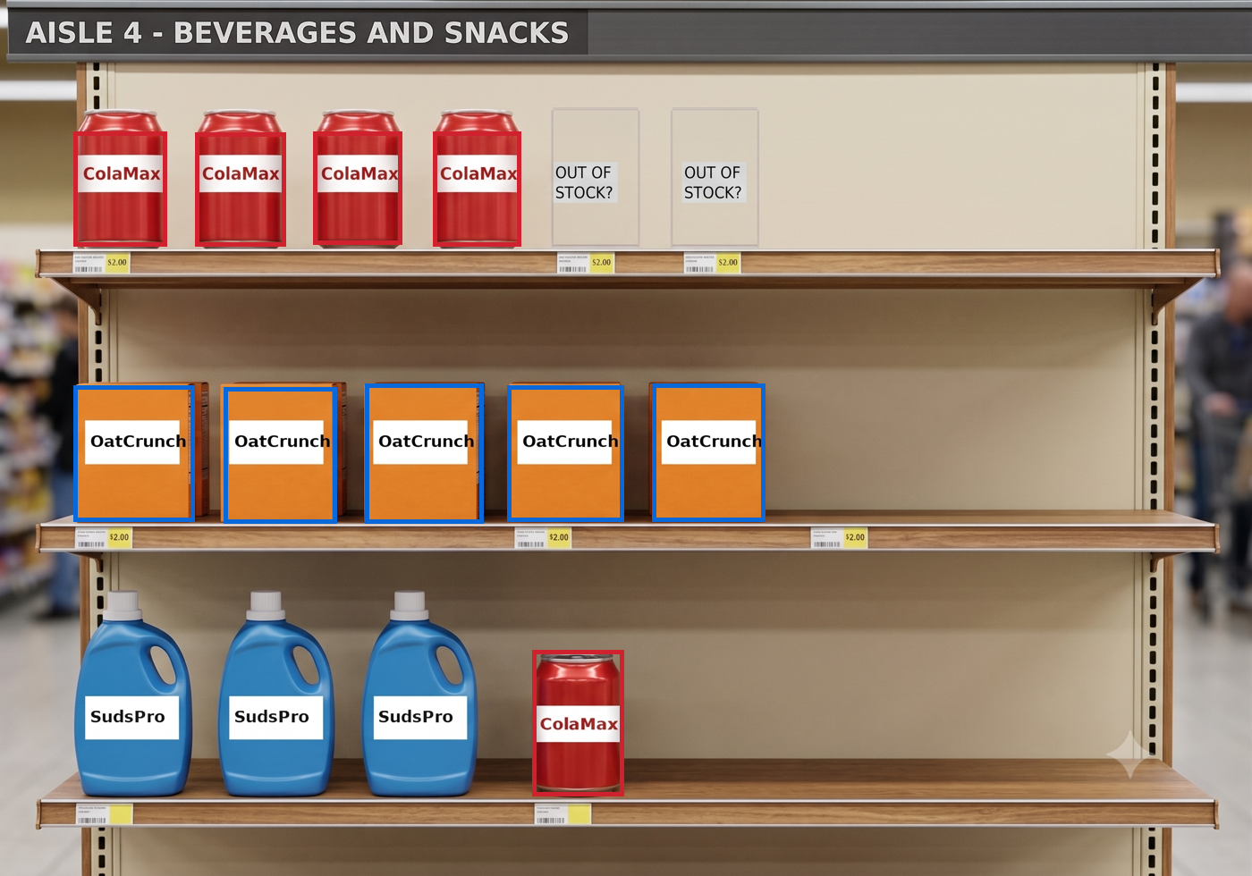
Boxes change what an evaluation can distinguish. A count of five ColaMax containers could be the right five, or four right plus one shelf tag mistaken for a can, and the count alone cannot tell you which, whereas the overlay can. This is also the bridge to the self-hosted detection models mentioned at the end of the chapter: a production shelf-audit system typically runs a dedicated detector for boxes at scale and reserves the language model for the questions detectors cannot answer.
19.5.2 The same audit on a crowded shelf
The clean render is the friendly case. Real aisles are packed, occluded, and stocked in depth, so we generated one of those as well, cluttered the way a photograph of a working aisle is.
shelf_real = (DATA_DIR / "images" / "shelf_real.png").read_bytes()
display(Image(shelf_real, width=640))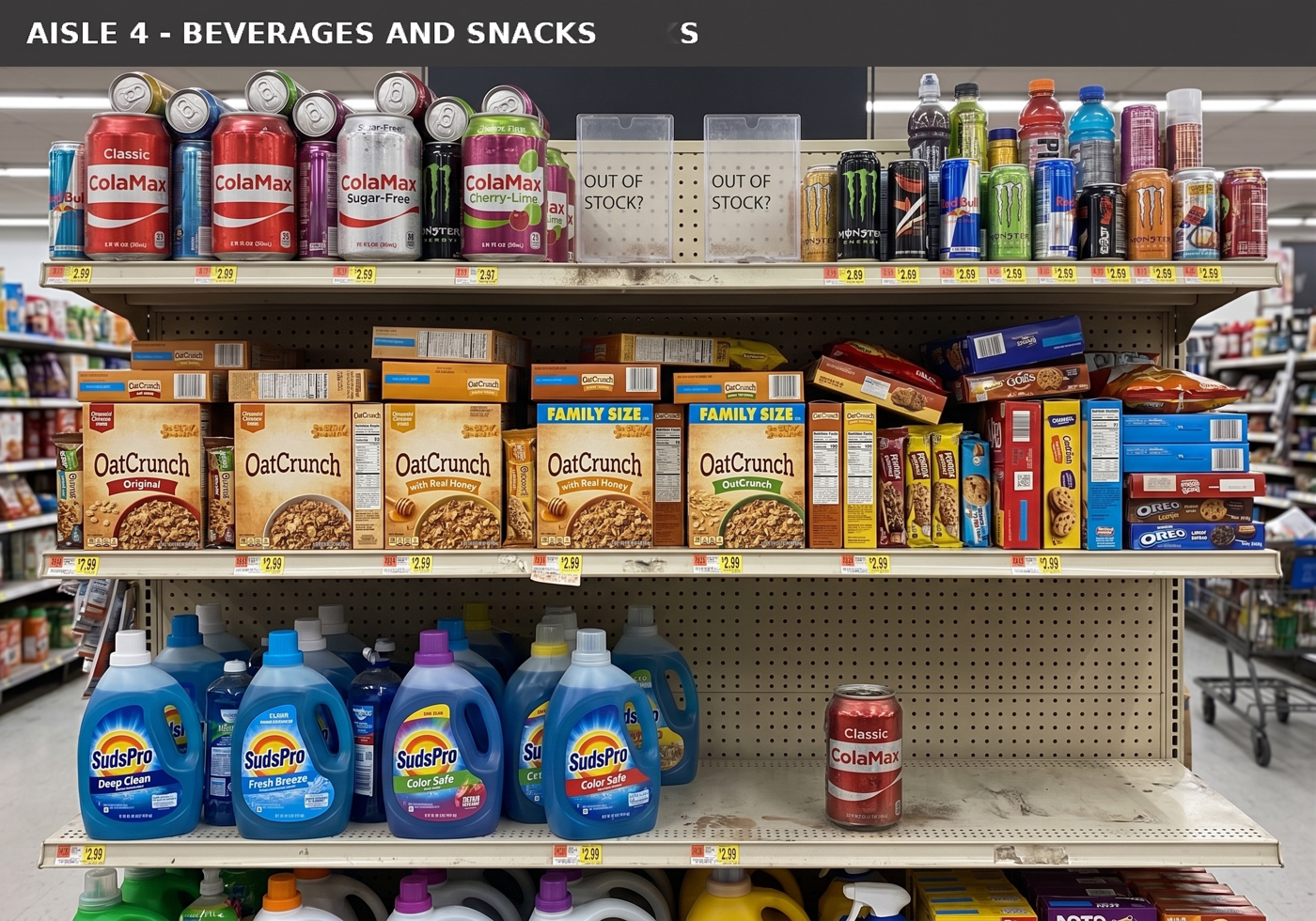
Our first instinct was to re-run the counting audit, and it taught us something better than a score: on a shelf like this, the counting question itself is broken. Products stand in rows behind rows, so “how many ColaMax” has no single right answer; our own hand counts changed depending on whether we counted facings, visible cans, or probable stock, and a gold label that the labelers cannot agree on cannot grade anyone. The tempting remedy, a stronger counter, would inherit the same undecidable gold; the practitioner’s move is a better question. Real planogram compliance works zone by zone: the planogram says which region of the shelf belongs to which product, and the questions become decidable. Does this product’s zone show an out-of-stock gap? Does any product that does not belong appear in it? We define the zones ourselves, in normalized coordinates, the way a real system gets them from the planogram, and we draw them so there is no ambiguity about what we are asking.
WarningDon’t outsource this
Deciding that the counting question itself is broken, and rewriting it as three decidable zone probes, is the judgment this shelf audit turns on. A coding tool will happily keep counting facings all afternoon and report a number for a shelf stocked in depth; seeing that the question has no defensible answer, and that the audit therefore needs a different structure entirely, requires you, looking at the crowded image and your own disagreeing hand counts. Redesigning the question is evaluation work, and it has to stay yours.
ZONES = {  # normalized (x0, y0, x1, y1): ours, from the planogram, not the model's
    "ColaMax":   (0.01, 0.05, 0.58, 0.31),
    "OatCrunch": (0.01, 0.41, 0.58, 0.62),
    "SudsPro":   (0.01, 0.62, 0.72, 0.95),
}
zone_img = PILImage.open(_io2.BytesIO(shelf_real)).copy()
zd = ImageDraw.Draw(zone_img)
ZW, ZH = zone_img.size
for zname, (x0, y0, x1, y1) in ZONES.items():
    zd.rectangle([x0*ZW, y0*ZH, x1*ZW, y1*ZH], outline="#bf8700", width=6)
    zd.text((x0*ZW + 10, y0*ZH + 8), zname, fill="#bf8700")
display(Image(_pil_bytes(zone_img), width=640))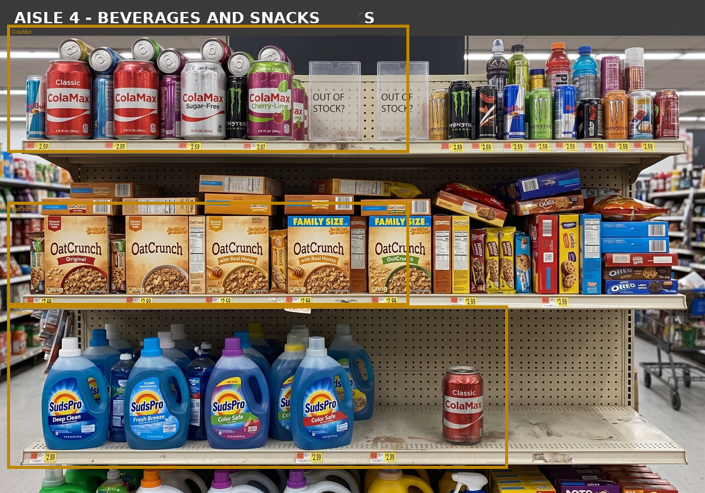
Each zone is cropped out and probed with the two questions, plus one whole-image question about misplaced products. Cropping is the simplest way to scope a model’s attention: the model cannot wander outside a region it never saw.
class ZoneProbe(BaseModel):
    empty_space_or_out_of_stock: bool
    foreign_product_present: bool
    foreign_product_description: str

def probe_zone(product: str, box) -> ZoneProbe:
    x0, y0, x1, y1 = box
    crop = PILImage.open(_io2.BytesIO(shelf_real)).crop(
        (int(x0*ZW), int(y0*ZH), int(x1*ZW), int(y1*ZH)))
    reply = call_vision(
        f"This is the {product} section of a store shelf. Two questions. "
        f"1: Is there empty shelf space or an out-of-stock marker in this section? "
        f"2: Is any product visible here that is not {product}? If so, what?",
        _pil_bytes(crop), max_tokens=200).text
    return call_structured("Extract the answers from this text:\n" + reply,
                           ZoneProbe).data

gz = json.loads((DATA_DIR / "images" / "vision_gold.json").read_text())["shelf_real"]["zones"]
rows = []
for product, box in ZONES.items():
    p = probe_zone(product, box)
    g = gz[product]
    rows.append({"zone": product, "probe": "gap / out-of-stock",
                 "gold": g["empty_space"], "model": p.empty_space_or_out_of_stock,
                 "hit": p.empty_space_or_out_of_stock == g["empty_space"]})
    rows.append({"zone": product, "probe": "foreign product",
                 "gold": g["foreign_product"], "model": p.foreign_product_present,
                 "hit": p.foreign_product_present == g["foreign_product"]})
    if p.foreign_product_present:
        print(f"{product}: foreign item reported: {p.foreign_product_description[:80]}")

whole = call_vision(
    "Looking at the whole shelf: is any product sitting in a section where it "
    "does not belong? If so, what and where?",
    shelf_real, max_tokens=150).text
print("\nwhole-shelf misplaced check:", whole[:160])
pd.DataFrame(rows)
ColaMax: foreign item reported: Monster Energy
OatCrunch: foreign item reported: Oat Crunch bar
SudsPro: foreign item reported: Classic ColaMax
whole-shelf misplaced check: Yes, the "Classic ColaMax" product is in a section where it does not belong. It is located on the bottom shelf, which is stocked with cleaning supplies (SudsPro| zone | probe | gold | model | hit | |
|---|---|---|---|---|---|
| 0 | ColaMax | gap / out-of-stock | True | True | True |
| 1 | ColaMax | foreign product | True | True | True |
| 2 | OatCrunch | gap / out-of-stock | False | True | False |
| 3 | OatCrunch | foreign product | True | True | True |
| 4 | SudsPro | gap / out-of-stock | True | True | True |
| 5 | SudsPro | foreign product | True | True | True |
The zone gold here is decidable in a way the counts never were: the ColaMax zone really does contain out-of-stock tags and a clutch of energy drinks wedged between the cans, and the SudsPro zone has both an empty stretch and the stray ColaMax can sitting in it. The OatCrunch zone taught us a lesson of its own. We labeled it clean on both probes; the model disagreed on the foreign-product question and named a slim snack box wedged between the cartons, and when we went back to the pixels at full resolution, the model was right, so the gold changed. This is gold labels working as intended: a disagreement is a trigger for re-inspection, and the correction sometimes falls on the labeler. A model that answers these zone questions correctly is auditing the shelf in the sense a retail team means it, and when either side misses, the miss names a zone and a question, where a count that was arguable to begin with would have absorbed it. The general lesson applies well beyond shelves: when a vision question has no defensible gold, change the question until the gold is decidable, because no amount of model tuning can make an undecidable label gradable.
19.6 Video is frames plus time
A security camera produces images with timestamps, which is no new kind of data, and that one idea makes video analytics buildable with everything already on the table: sample frames, extract a number from each, and you have a time series. Our clip is an AI-generated security-camera sequence, twelve photorealistic frames at two-minute intervals showing a checkout queue build and drain. We watched every frame and hand-labeled the queue length, customers only, cashier excluded, because a counting rule you never wrote down is a disagreement waiting for deployment. The labels make the extraction scorable.
from PIL import Image as PILImage, ImageSequence
import io as _io

clip = PILImage.open(DATA_DIR / "video" / "checkout.gif")
frames = [f.convert("RGB") for f in ImageSequence.Iterator(clip)]
print(f"{len(frames)} frames, {frames[0].size[0]}x{frames[0].size[1]}")

fig, axes = plt.subplots(1, 3, figsize=(9.5, 2.1))
for ax, idx in zip(axes, [0, 6, 11]):
    ax.imshow(frames[idx]); ax.set_title(f"frame {idx} (14:{18 + 2*idx:02d})", fontsize=9)
    ax.axis("off")
plt.tight_layout(); plt.show()
12 frames, 640x358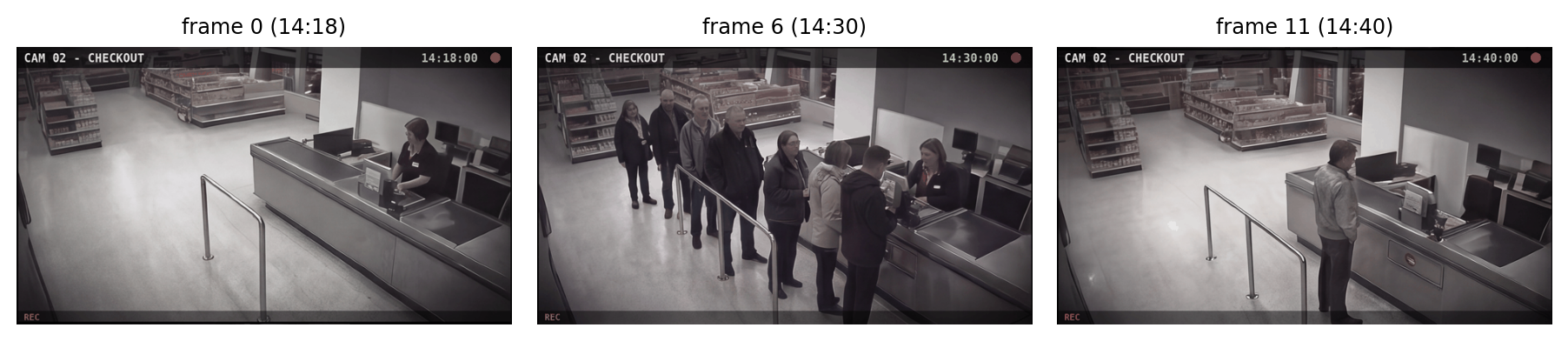
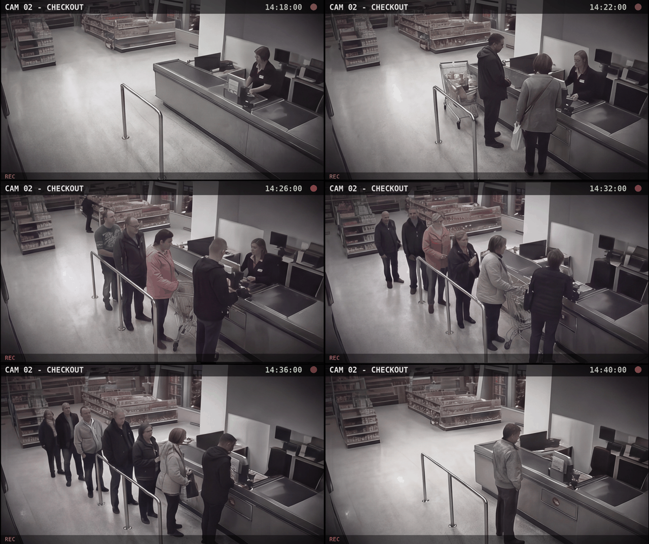
With twelve frames we read every one, asking one narrow question per frame and demanding a bare number back. At a real camera’s frame rate you would sample instead, and the Evaluate lab measures that trade. The counting rule is stated in the prompt, because the model cannot follow a rule we never state.
import re
import pandas as pd

def frame_bytes(f) -> bytes:
    buf = _io.BytesIO(); f.save(buf, format="PNG"); return buf.getvalue()

sampled = list(range(len(frames)))
counts = []
for i in sampled:
    reply = call_vision("How many customers are waiting or being served at the "
                        "checkout? Do not count the cashier. "
                        "Reply with only the number.",
                        frame_bytes(frames[i]), max_tokens=10).text
    m = re.search(r"\d+", reply)
    counts.append(int(m.group()) if m else -1)

gold_q = json.loads((DATA_DIR / "images" / "vision_gold.json").read_text())["video"]["queue_per_frame"]
minutes = [i * 2 for i in sampled]
pd.DataFrame({"minute": minutes, "model count": counts,
"true count": [gold_q[i] for i in sampled]})| minute | model count | true count | |
|---|---|---|---|
| 0 | 0 | 1 | 0 |
| 1 | 2 | 4 | 3 |
| 2 | 4 | 2 | 2 |
| 3 | 6 | 3 | 3 |
| 4 | 8 | 5 | 4 |
| 5 | 10 | 6 | 6 |
| 6 | 12 | 7 | 7 |
| 7 | 14 | 6 | 6 |
| 8 | 16 | 6 | 7 |
| 9 | 18 | 6 | 7 |
| 10 | 20 | 7 | 6 |
| 11 | 22 | 1 | 1 |
fig, ax = plt.subplots(figsize=(6.5, 3.6))
ax.plot(minutes, [gold_q[i] for i in sampled], color="#9a9a9a",
        linewidth=1.5, label="true (hand-labeled)")
ax.plot(minutes, counts, marker="o", color="#0969da", label="model count")
ax.axhline(5, color="#cf222e", linestyle="--", linewidth=1, label="staffing threshold")
ax.set_xlabel("minute"); ax.set_ylabel("people in queue")
ax.legend(frameon=False)
ax.spines[["top", "right"]].set_visible(False)
plt.tight_layout(); plt.show()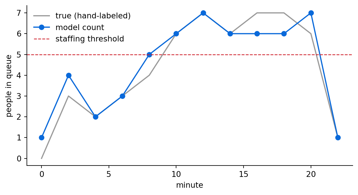
errors = [abs(c - gold_q[i]) for c, i in zip(counts, sampled) if c >= 0]
over = [m for m, c in zip(minutes, counts) if c >= 5]
print(f"mean absolute count error: {sum(errors)/len(errors):.2f}")
print("threshold (5+) first crossed at minute:", over[0] if over else "never")
mean absolute count error: 0.50
threshold (5+) first crossed at minute: 8This is video analytics in one page: frames, a per-frame extraction, a time series, an event. Two notes for the real version. Sampling rate sets the cost: a frame every few seconds for a queue, every frame for a safety-critical line, and each sampled frame is one image-priced call. And whereas our clip is a GIF, real files are mp4 streams; ffmpeg or OpenCV pulls frames with one call (ffmpeg -i camera.mp4 frames/f_%d.jpg) and everything downstream is identical.
19.6.1 Sending the video itself
The per-frame pipeline is no longer the only option. Current multimodal models accept video as a first-class input, the way they accept images, and reason over the frames and their order in one call. Qwen’s VL models handle video natively, as do Gemini’s; through the same API we have used all along, we can send the clip as one content part.
import base64

video_b64 = base64.b64encode(
    (DATA_DIR / "video" / "checkout.mp4").read_bytes()).decode()

from gaba.llm import get_client

reply = get_client().chat.completions.create(
    model="qwen/qwen3.6-35b-a3b",   # video-capable; Gemini models also accept video
    messages=[{"role": "user", "content": [
        {"type": "text", "text":
         "This is a checkout security camera clip with a timestamp in each "
         "frame. Describe how the queue length changes over the clip: when "
         "does it peak, roughly how many customers at the peak (do not count "
         "the cashier), and when does a second register become justified if "
         "the threshold is five?"},
        {"type": "video_url",
         "video_url": {"url": f"data:video/mp4;base64,{video_b64}"}},
    ]}],
    max_tokens=1200,
    extra_body={"reasoning": {"enabled": False}},
)
print(reply.choices[0].message.content[-700:])
print(f"\n[whole clip: {reply.usage.prompt_tokens} prompt tokens]")
er continues to serve the customers one by one.
### Summary:
- **Peak Queue Length**: The queue peaks at 14:28:00 with five customers (excluding the cashier).
- **Justification for Second Register**: A second register becomes justified when the queue reaches five customers, which occurs at 14:28:00.
Thus, the queue length changes as follows:
- Starts with 1 customer at 14:20:00.
- Increases to 2 customers at 14:22:00.
- Increases to 3 customers at 14:24:00.
- Increases to 4 customers at 14:26:00.
- Peaks at 5 customers at 14:28:00.
- Remains at 5 customers from 14:28:00 to 14:40:00.
The second register should be justified at 14:28:00 when the queue reaches the threshold of five customers.
[whole clip: 1437 prompt tokens]Score this against the gold labels and the per-frame table above before deciding it has replaced the pipeline. In the runs we have watched, the one-call version reliably reports the story correctly, an empty register, a build, a peak, a drain, and it cites the on-frame timestamps, which the per-frame pipeline never even saw as text. Its precise counts are less exact: peaks come back a head or two off and threshold crossings drift a frame, errors you can only detect because the per-frame pipeline and the hand labels exist. This is the trade: native video provides temporal reasoning in one cheap call (the entire clip cost fewer prompt tokens than two of our single frames), while giving up the per-frame numbers you could audit. For a narrative answer, send the video; for a dashboard, keep the pipeline; for production, the strong pattern is both, the cheap native call to triage which clips deserve the per-frame treatment.
Two adjacent capabilities lie outside this book’s scope. Vision models also read screenshots and application interfaces, and computer-use agents go a step further, clicking and typing in a live user interface based on what they see, an agent pattern with its own safety questions that lies outside the extraction pipelines this chapter builds. And for search over visually rich corpora, visual-document retrieval embeds page images directly with ColPali-style multimodal embeddings, the direction adjacent to retrieval-augmented generation (RAG) to watch if your documents are scanned pages that offer no clean text. There is also a self-hosted route: open vision models run object detection from a text description (OWL-ViT) and visual question answering (BLIP) on your own GPU, and at millions of frames the Chapter 4 economics that favored the API begin to flip.
19.7 Evaluation: how accurate is the reading?
We can measure the reading against the values we put in the chart, and the measurement makes the labeled-versus-unlabeled distinction concrete.
Metric: how many of the four revenue figures the model reads within 5 percent of the true value. A relative tolerance is the right choice here: five billion dollars of slack would be invisible on the 412-billion bar and absurd on the 3-billion one.
Test set: the four companies, whose true revenues we set ourselves.
Baseline: the labeled chart, where near-exact reading should be easy; the unlabeled chart is the harder case.
To score the replies we need the four numbers out of the model’s free text; because regexing for digits and hoping the order holds is fragile, we use the same read-then-parse pattern as the invoice.
class ChartReading(BaseModel):
    northwind: float
    cascadia: float
    bluepeak: float
    harborlight: float

rows, readings = [], {}
for with_labels in [False, True]:
    reply = call_vision("List each company and its revenue value, one per line.",
                        revenue_chart(with_labels=with_labels)).text
    reading = call_structured(
        "Extract each company's revenue in billions from this text:\n" + reply,
        ChartReading,
    ).data
    readings["labeled" if with_labels else "unlabeled"] = reading
    got = [reading.northwind, reading.cascadia, reading.bluepeak,
           reading.harborlight]
    within = sum(abs(g - t) / t < 0.05 for g, t in zip(got, revenues))
    rows.append({"chart": "labeled" if with_labels else "unlabeled",
                 "read within 5% of true": f"{within}/4"})
pd.DataFrame(rows)| chart | read within 5% of true | |
|---|---|---|
| 0 | unlabeled | 2/4 |
| 1 | labeled | 4/4 |
The same readings, broken out per company, put the whole chapter in one figure.
import numpy as np

x = np.arange(len(companies))
fig, ax = plt.subplots(figsize=(7, 4))
for offset, (name, color) in zip([-0.2, 0.2],
                                 [("unlabeled", "#cf222e"), ("labeled", "#0969da")]):
    r = readings[name]
    got = [r.northwind, r.cascadia, r.bluepeak, r.harborlight]
    # exact reads have zero error, which a log axis cannot draw; floor at 0.01%
    rel = [max(abs(g - t) / t, 1e-4) for g, t in zip(got, revenues)]
    ax.bar(x + offset, rel, width=0.4, color=color, label=name)
ax.set_yscale("log")
ax.set_xticks(x, companies)
ax.axhline(0.05, color="#57606a", linestyle="--", linewidth=1)
ax.text(len(companies) - 1.45, 0.06, "5% tolerance", fontsize=8, color="#57606a")
ax.set_ylabel("relative error |read - true| / true")
ax.legend(frameon=False)
ax.spines[["top", "right"]].set_visible(False)
plt.tight_layout(); plt.show()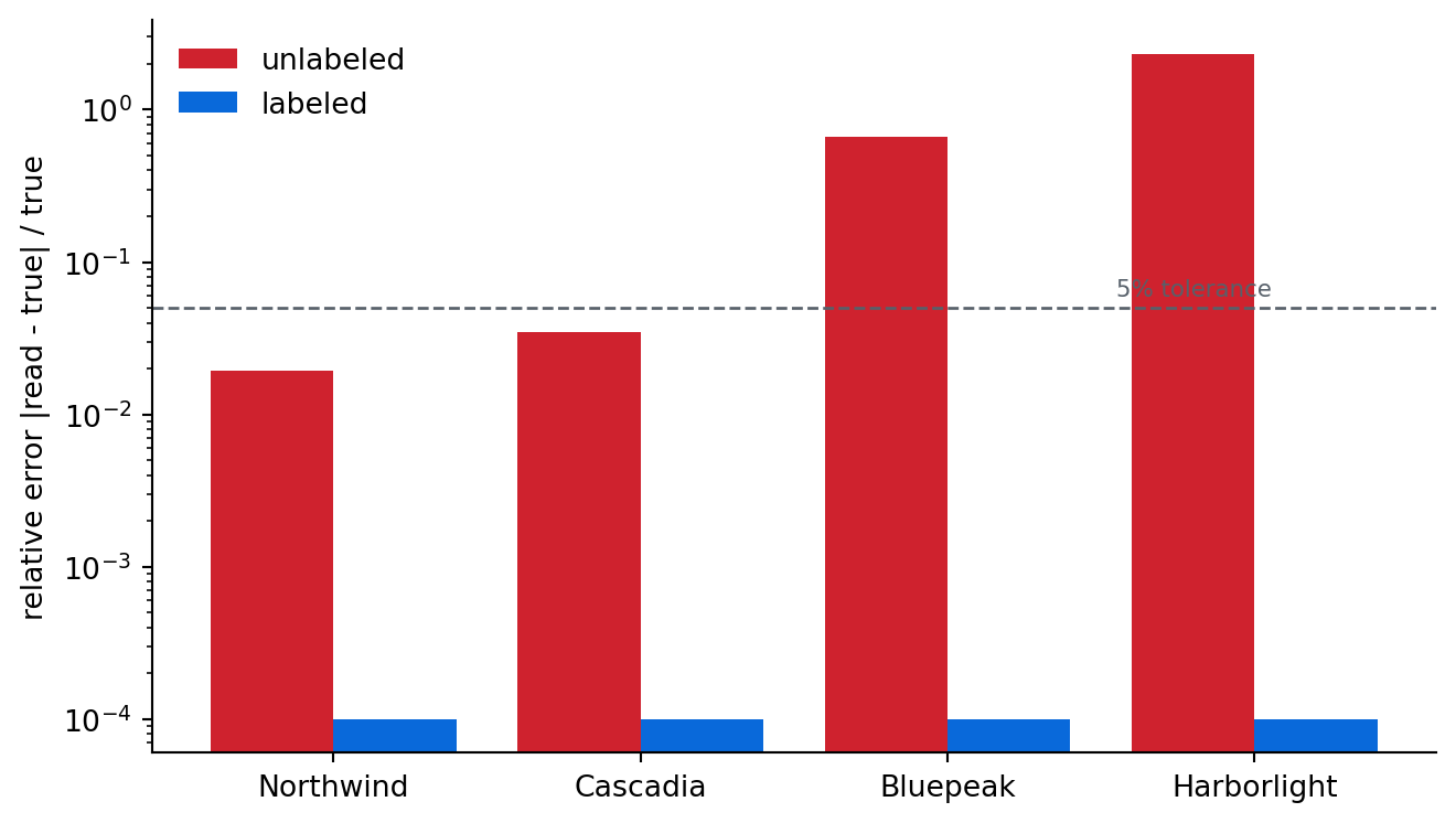
The labeled chart is read accurately; the unlabeled one is read approximately, sometimes within tolerance and sometimes not. This difference is the whole lesson of the chapter in one comparison. When you deploy a vision model on documents, design the task around what it reads exactly: point it at the printed numbers, because a picture of a quantity yields only an estimate. And evaluate it the same way you evaluate any extraction, against values you can verify, because a confident misreading of a chart is just as silent as a confident wrong answer from a text model.
TipCost: images cost more tokens than text
Most providers bill an image as a block of tokens that scales with its resolution, often more than a paragraph of text, so vision calls cost more than text calls. For a few documents the difference is negligible; for a pipeline reading millions of pages it accumulates quickly, and the remedy is the same as everywhere else: use the cheap multimodal model by default and reserve a stronger one for the documents it genuinely struggles with. The same arithmetic governs the self-hosted vision models named above, where the cost of a higher resolution or a faster sampling rate appears as GPU time and throughput, and the Chapter 4 economics decide when that route wins. Video multiplies this by the sampling rate; one frame every two minutes cost us nine calls, while one frame per second would cost thousands per hour of footage.
ImportantCompliance: document images carry everything on the page
A scanned invoice or form contains every field on the page, including fields you never asked about and often personal data such as signatures and account numbers. Sending the image to a model sends all of it. Camera footage is stricter still: video of identifiable people is personal data in most regimes, and analyzing it can trigger employee-monitoring and surveillance rules on top of the usual ones. The redaction and residency questions from Appendix D apply to the whole image, and to every frame.
19.8 Exercises
19.8.1 Conceptual questions
A vision model reads an unlabeled bar chart. Its values are best described as:
- Estimates, gauged from each bar’s apparent height against the axis
- Exact figures, since the model can measure each bar pixel by pixel
- Copies of the underlying data the chart was originally rendered from
- Random guesses anchored to nothing but the title and the axis labels
Vision-language models are most reliable when reading:
- Unlabeled quantities, such as the height of a bar or the slope of a line
- Color encodings, which map cleanly onto the model’s internal features
- Text and labels printed in the image, such as line items and totals
- Hand-drawn forms, which carry less visual noise than rendered charts
In the shelf audit, counting facings is harder for a vision model than reading a product label because counting requires:
- A higher-resolution image than label reading does
- Locating every instance without merging neighbors or counting one twice
- Packaging fonts that vision models are trained to recognize
- A context window large enough to hold one token per object
Why do vision calls usually cost more than text calls?
- Vision models run on separate, more expensive hardware than text-only models
- Each image must be uploaded twice, once for encoding and once with the question
- Providers bill vision by seconds of processing time, without counting output tokens
- An image is billed as a block of tokens that grows with the image’s resolution
The chapter turns camera footage into a queue trend by:
- Sending the whole clip to the model in a single call and asking for a summary
- Measuring pixel change between consecutive frames to infer motion
- Sampling frames, extracting one count per frame, and assembling them into a time series
- Reading the camera’s embedded metadata, which records the queue length
A vision model confidently misreads a chart value. The chapter calls this dangerous because the failure is:
- Silent, exactly like a confident wrong answer from a text model
- Contagious, corrupting every later call made in the same session
- Costly, since every retry doubles the token price of the request
- Rare enough that no validation step will ever surface it in testing
The practical rule for using vision on business documents is to:
- Reserve the strongest available model for every page, since the errors are silent
- Convert every image to plain text with a separate OCR (optical character recognition) tool and never send the image
- Ask the model to estimate depicted quantities, since estimation is its core strength
- Point it at what is written on the page and verify against values you can check
Why does compliance apply to the whole image of a scanned invoice?
- Image files embed location metadata that a model can read back out of the pixels
- Sending the image sends every field on the page, signatures and account numbers included
- Vision providers retain images for longer than they retain ordinary text prompts
- Scanned documents count as legal originals, so transmitting one transfers custody
19.8.2 Build lab
Render a small table of numbers as an image (using matplotlib text or a screenshot of a dataframe) and extract it with call_vision into a structured form. Check the extracted values against the source. Report whether reading a table image is closer to the labeled-chart case or the unlabeled-chart case, and why.
19.8.3 Evaluate lab
The chapter read every frame of the twelve-frame clip. Re-run the queue extraction sampling every second frame and every third frame, scoring each run against the gold counts in vision_gold.json, and note where the sparser runs miss or delay the threshold crossing. Report the accuracy and the number of vision calls for all three rates, then write two sentences recommending a rate for a camera that produces a frame every two seconds, trading detection delay against cost, the same cost-quality judgment as every other chapter.
NoteWhere we go next
Images are static. Chapter 20 turns to data that moves through time, such as sales, demand, and prices, and uses a foundation model built for forecasting to predict the future of a series it has never seen, the last of the three beyond-text chapters.