import numpy as np
import torch
import matplotlib.pyplot as plt20 Time-series forecasting with foundation models
Predicting a series the model has never seen
Forecasting is one of the oldest jobs in business analytics: how much will we sell next quarter, what will demand be, where are prices heading. The traditional approach is to train a model on each series. This could be an ARIMA (autoregressive integrated moving average) or a Prophet fit, or any other classical statistical forecaster. This means we have a great many models to build and maintain, with one model per product, per store, per metric. Time-series foundation models remove this per-series training step. A model like Chronos, Amazon’s time-series foundation model, is pretrained on an enormous collection of series. When it comes time to forecast a new series that it has never seen, it does so with no training at all, the same zero-shot move that language models made for text. In this chapter, we forecast a business series with one, reading the uncertainty it reports and measuring it against a naive baseline.
NoteIn the running system
Once our desk is handling the ticket queue, the next question is how much work is coming and when. This chapter forecasts a business series, such as weekly ticket volume, so the system can be staffed and budgeted in advance, whereas a desk without a forecast can only react to the volume that arrives.
NoteSetup for this chapter
Run in the gaba-core environment. This chapter uses Chronos, a time-series foundation model. A small variant downloads on a first run and forecasts on CPU in well under a second. No API key is needed.
20.1 A series to forecast
We use a synthetic monthly sales series with the structure real business series have: an upward trend, a yearly seasonal cycle, and noise. We hold out the last twelve months to forecast and check against.
np.random.seed(0)
months = np.arange(48)
sales = 100 + months * 2 + 15 * np.sin(2 * np.pi * months / 12) + np.random.normal(0, 5, 48)

context, actual = sales[:36], sales[36:]  # train on 36 months, forecast 12
print(f"{len(context)} months of history, forecasting {len(actual)} ahead")
36 months of history, forecasting 12 ahead20.2 Zero-shot forecasting
We load Chronos (specifically chronos-bolt-small, Chronos-Bolt being the faster successor to the original Chronos) and ask it to forecast. There is no training step here, as the model was pretrained on many series and now applies that knowledge to ours directly. Chronos returns a probabilistic forecast, a set of quantiles (cutoffs like the 10th and 90th percentile) whose spread expresses uncertainty in a way that a single forecast line cannot.
flowchart LR
    hist["Historical series<br/>(36 months of sales)"] --> fm["Chronos<br/>pretrained foundation model<br/>no training on this series"]
    fm --> prob["Probabilistic forecast<br/>(quantiles for the<br/>next 12 months)"]
    hist -.-> fit["Fit SARIMA to<br/>this exact series first"]
    fit -.-> cls["Classical forecast"]
from chronos import BaseChronosPipeline

pipe = BaseChronosPipeline.from_pretrained("amazon/chronos-bolt-small",
                                           device_map="cpu", dtype=torch.float32)

quantiles, mean = pipe.predict_quantiles(
    torch.tensor(context, dtype=torch.float32),
    prediction_length=12,
    quantile_levels=[0.1, 0.5, 0.9],
)
forecast = mean[0].numpy()
low = quantiles[0, :, 0].numpy()   # 10th percentile
high = quantiles[0, :, 2].numpy()  # 90th percentile
print("forecast (next 12 months):", np.round(forecast, 1))
forecast (next 12 months): [166.9 172.5 177.9 180.5 178.7 173.1 165.2 156.2 150.8 150.7 153.8 158. ]20.3 Seeing the forecast and its uncertainty
A forecast without a sense of its uncertainty is only half a forecast. Chronos gives us a band, called a prediction interval, that represents the range within which it expects the true value to fall most of the time. Plotting it shows how the band behaves: confident in the near term, widening as it reaches further out.
fig, ax = plt.subplots(figsize=(9, 4))
ax.plot(months[:36], context, label="history", color="#57606a")
ax.plot(months[36:], actual, label="actual", color="#1f2328", marker="o", markersize=3)
ax.plot(months[36:], forecast, label="forecast", color="#0969da")
ax.fill_between(months[36:], low, high, alpha=0.2, color="#0969da",
                label="80% interval")
outside = (actual < low) | (actual > high)
ax.plot(months[36:][outside], actual[outside], "x", color="#cf222e",
        markersize=9, markeredgewidth=2, label="outside the band", zorder=5)
ax.axvline(35, color="#9a9a9a", linestyle=":")
ax.set_xlabel("month"); ax.set_ylabel("sales")
ax.legend(frameon=False)
ax.spines[["top", "right"]].set_visible(False)
plt.tight_layout(); plt.show()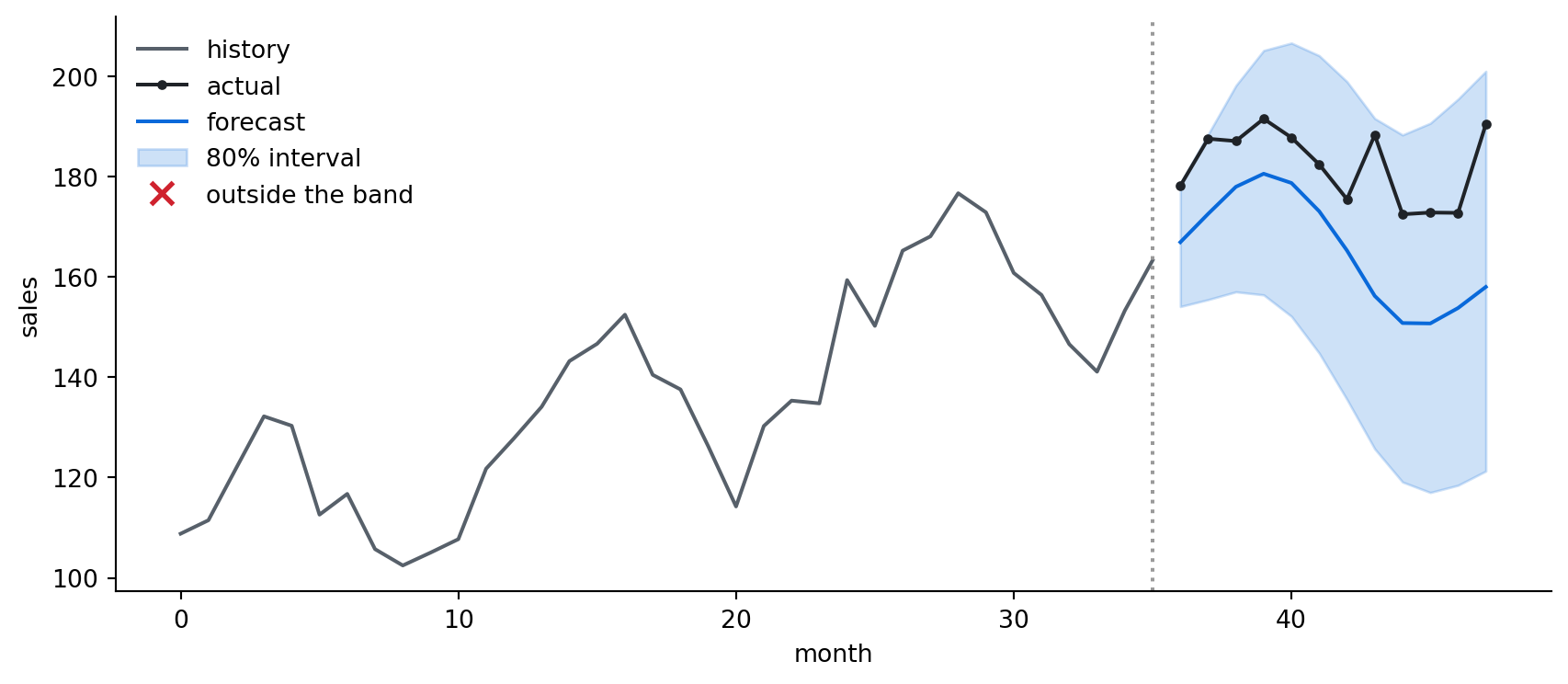
The forecast tracks the trend and the seasonal rise and fall, and the band widens with the horizon, which is the behavior you want: the model is more certain about next month than about a year out, and it reports that openly. For a business decision, that band is often more valuable than the central line, because it tells you the range you must plan for.
A band also makes a checkable claim: an 80 percent interval should contain roughly four of every five actuals.
inside = (actual >= low) & (actual <= high)
print(f"band coverage: {inside.mean():.0%} of the 12 held-out months "
      f"(nominal: 80%)")
print(f"band width at h=1: {high[0] - low[0]:.1f}   at h=12: {high[-1] - low[-1]:.1f}")
band coverage: 100% of the 12 held-out months (nominal: 80%)
band width at h=1: 24.5 at h=12: 79.7The width line quantifies the visible flaring: the model commits to a much tighter range one month out than twelve. The coverage line should be quoted with a caveat: with only twelve months, one actual in or out moves coverage by eight points. This is a sanity check that the band is roughly right, but a calibration measurement, which asks whether an 80 percent band actually contains about 80 percent of the actual values over many cases, requires many series or many windows, which is exactly what the scale experiment later in the chapter provides the raw material for.
20.4 Evaluation: does it beat doing nothing?
A forecast is only useful if it beats the cheapest alternative. The cheapest forecast is the naive one, the assumption that next month will look like this month, so that is our baseline.
Metric: mean absolute error, MAE (the average size of the forecast’s misses) against the held-out actuals.
Test set: the twelve months we held out.
Baselines: the naive forecast (repeat the last value), and a classical SARIMA (seasonal ARIMA) model fitted to this exact series, which is the stronger alternative a foundation model must be measured against.
import pandas as pd
import warnings
warnings.filterwarnings("ignore")
from statsmodels.tsa.statespace.sarimax import SARIMAX

mae = lambda p: np.mean(np.abs(p - actual))

naive_forecast = np.full(12, context[-1])
sarima = SARIMAX(context, order=(1, 1, 1), seasonal_order=(1, 1, 0, 12)).fit(disp=False)
sarima_forecast = sarima.forecast(12)

pd.DataFrame({
    "method": ["Chronos (zero-shot)", "naive (last value)", "SARIMA (fitted)"],
    "MAE": [round(mae(forecast), 1), round(mae(naive_forecast), 1),
            round(mae(sarima_forecast), 1)],
})| method | MAE | |
|---|---|---|
| 0 | Chronos (zero-shot) | 16.8 |
| 1 | naive (last value) | 18.9 |
| 2 | SARIMA (fitted) | 6.5 |
The same comparison as a chart makes the gap easier to see.
methods = ["Chronos\n(zero-shot)", "naive\n(last value)", "SARIMA\n(fitted)"]
errors = [mae(forecast), mae(naive_forecast), mae(sarima_forecast)]

fig, ax = plt.subplots(figsize=(6, 4))
bars = ax.bar(methods, errors, color=["#0969da", "#cf222e", "#8250df"])
for bar, err in zip(bars, errors):
    ax.text(bar.get_x() + bar.get_width() / 2, err, f"{err:.1f}",
            ha="center", va="bottom")
ax.set_ylabel("MAE on held-out months")
ax.spines[["top", "right"]].set_visible(False)
plt.tight_layout()
plt.show()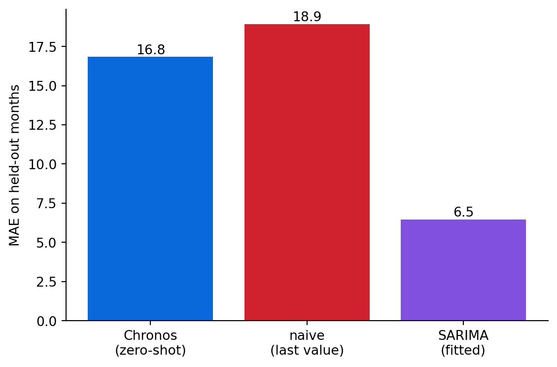
Read together, the three rows give a more complete result than “Chronos wins.” Chronos beats the naive baseline without ever being trained on this series, so a single pretrained model forecasts a new series straight out of the box. But a classical SARIMA model, fitted to this exact series, beats Chronos decisively, and this comparison favors SARIMA by construction: our synthetic series is trend plus sinusoidal seasonality plus Gaussian noise, which is exactly the data-generating process SARIMA assumes, and we supplied the seasonal period of twelve; on messier real series, where the structure is less textbook, the gap narrows. The direction of the result is neither a surprise nor a mark against Chronos. On one clean, well-behaved series, given the time to fit a model to it, a model fitted to that series wins. The foundation model’s advantage lies in scale without fitting, since accuracy on any single clean series, as we have just seen, favors the model fitted to it. Building and tuning ten thousand SARIMA models is a substantial engineering effort; one Chronos forecasts ten thousand series with no training at all. So reach for the foundation model when you have more series than you can fit individually, or series too irregular for a classical model to capture, and reach for the fitted classical model when you have a clean series and the time to fit it. The only way to know which case you are in is the comparison we just ran, on your data.
The model family as it stands in 2026 is broader than Chronos-Bolt, which is one member of a now-crowded field: Chronos-2 extends the approach to multivariate forecasting and covariates (outside drivers like promotions or holidays), and TimesFM (Google) and Moirai (Salesforce) are credible peers worth including in any comparison. That matters because the pipeline we demonstrated is univariate, the model sees only the sales history itself, and that is its biggest practical limitation. Real demand moves with promotions, price changes, and holidays, and a forecaster that cannot take those covariates as input leaves known information unused. If your forecasts hinge on such drivers, look at the covariate-capable members of the family, and run the same held-out comparison before committing.
TipCost: a forecast is almost free
Chronos runs locally and forecasts in a fraction of a second, so the marginal cost of a forecast is negligible, and there is no per-series training cost at all. That changes the economics of forecasting at scale: where fitting ten thousand ARIMA models was a substantial engineering effort, one foundation model forecasts ten thousand series with no training, and you spend your effort on evaluating which series it serves well, with no need to build a model for each.
The callout’s claim is arithmetic, so here is the arithmetic with your numbers in it. Although compute is the obvious cost, the fitted-model cost that matters is the analyst minutes each series demands to fit, validate, and maintain, multiplied by how many series there are and how often they refresh.
20.5 One hundred series at once
The scale argument deserves a measurement to stand beside the arithmetic above. We generate one hundred synthetic monthly series with randomized trends, seasonal strengths, and noise levels, and give a third of them a mid-series slope break, which is the kind of structural change that real demand series undergo and fixed-form models handle poorly. Then both contenders forecast all hundred: Chronos zero-shot in a loop, and a fresh SARIMA fitted to each series, with the order held fixed because nobody hand-tunes ten thousand models.
import time

rng_scale = np.random.default_rng(42)
series_list, has_break = [], []
for i in range(100):
    t = np.arange(48)
    y = (100 + rng_scale.uniform(-1.5, 3.0) * t
         + rng_scale.uniform(0, 20) * np.sin(2 * np.pi * t / 12 + rng_scale.uniform(0, 2 * np.pi))
         + rng_scale.normal(0, rng_scale.uniform(2, 10), 48))
    if i < 33:   # a third get a mid-series slope break
        kink = int(rng_scale.integers(18, 30))
        y[kink:] += rng_scale.uniform(-2.5, 2.5) * np.arange(48 - kink)
    series_list.append(y)
    has_break.append(i < 33)
has_break = np.array(has_break)

t0 = time.perf_counter()
chronos_maes = []
for y in series_list:
    _, m = pipe.predict_quantiles(torch.tensor(y[:36], dtype=torch.float32),
                                  prediction_length=12, quantile_levels=[0.5])
    chronos_maes.append(float(np.mean(np.abs(m[0].numpy() - y[36:]))))
chronos_seconds = time.perf_counter() - t0

t0 = time.perf_counter()
sarima_maes, failures = [], 0
for y in series_list:
    try:
        fit = SARIMAX(y[:36], order=(1, 1, 1),
                      seasonal_order=(1, 1, 0, 12)).fit(disp=False)
        pred = fit.forecast(12)
    except Exception:           # a fit that blows up falls back to naive
        pred, failures = np.full(12, y[35]), failures + 1
    sarima_maes.append(float(np.mean(np.abs(pred - y[36:]))))
sarima_seconds = time.perf_counter() - t0

chronos_maes, sarima_maes = np.array(chronos_maes), np.array(sarima_maes)
print(f"Chronos: {chronos_seconds:.0f}s for 100 series | "
      f"SARIMA: {sarima_seconds:.0f}s for 100 series ({failures} failed fits)")
print(f"median MAE, smooth series:  Chronos {np.median(chronos_maes[~has_break]):.1f}  "
      f"SARIMA {np.median(sarima_maes[~has_break]):.1f}")
print(f"median MAE, break series:   Chronos {np.median(chronos_maes[has_break]):.1f}  "
      f"SARIMA {np.median(sarima_maes[has_break]):.1f}")
Chronos: 1s for 100 series | SARIMA: 4s for 100 series (0 failed fits)
median MAE, smooth series: Chronos 10.4 SARIMA 6.4
median MAE, break series: Chronos 13.9 SARIMA 11.6diff = chronos_maes - sarima_maes # positive: SARIMA was better on that series
fig, ax = plt.subplots(figsize=(7, 4))
for mask, label, color in [(~has_break, "smooth series", "#0969da"),
(has_break, "slope-break series", "#cf222e")]:
vals = np.sort(diff[mask])
ax.plot(vals, np.arange(1, len(vals) + 1) / len(vals),
drawstyle="steps-post", color=color, label=label)
ax.axvline(0, color="#57606a", linewidth=1, linestyle="--")
ax.set_xlabel("per-series MAE difference (Chronos minus SARIMA)")
ax.set_ylabel("fraction of series")
ax.legend(frameon=False)
ax.spines[["top", "right"]].set_visible(False)
plt.tight_layout(); plt.show()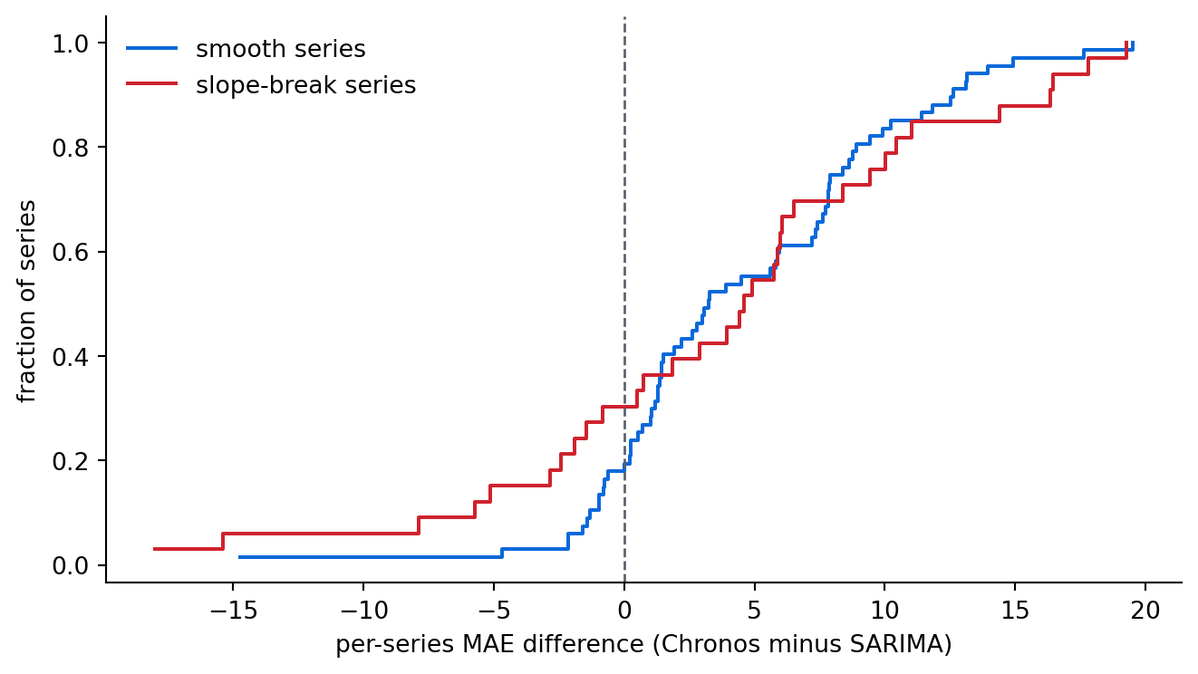
The chart reads in both directions. On the smooth series the fitted model tends to win, just as it did on the single clean series earlier: when a series matches SARIMA’s assumptions, fitting to it improves accuracy. The slope-break series narrow that gap or flip it, because a break violates the fixed-form assumptions while the foundation model, pretrained on a vast variety of series, treats a kink as just another pattern. And the wall clock is the third result: the fitting loop took many times longer than the zero-shot loop on one hundred series, and at ten thousand series that multiplier becomes the difference between an afternoon and a standing engineering commitment, before counting the per-series attention the calculator above prices. The accuracy argument favors fitting clean series, the economics argument favors zero-shot portfolios, and the experiment shows which case applies to your data.
20.6 When the future depends on things you know
The comparison above had one advantage for every model: nothing outside the series itself drove the numbers. Real business series are rarely so self-contained. Sales spike when marketing runs a promotion, demand moves with holidays and price changes, and, crucially, the business knows its own promotion calendar in advance. A forecaster that cannot accept that knowledge leaves known information unused. This is the covariate limitation we flagged earlier; now we measure what it costs.
The series below has the same trend-plus-seasonality structure with one addition: in promotion months, sales jump by roughly forty units. Four of the twelve held-out months are promotion months, and we know which ones, because we scheduled them.
rng = np.random.default_rng(1)
promo = np.zeros(48)
promo[[6, 11, 17, 23, 29, 35, 38, 41, 44, 47]] = 1.0   # the promo calendar
sales_p = (100 + months * 2 + 15 * np.sin(2 * np.pi * months / 12)
           + 40 * promo + rng.normal(0, 5, 48))

ctx_p, act_p = sales_p[:36], sales_p[36:]
promo_ctx, promo_future = promo[:36], promo[36:]
print(f"promo months in the held-out year: {int(promo_future.sum())} of 12")
promo months in the held-out year: 4 of 12Chronos sees only the history. SARIMAX sees the history as well as the promotion flag (including the future flags), which is fair because a promotion calendar is exactly the kind of future a business knows.
q_p, mean_p = pipe.predict_quantiles(
    torch.tensor(ctx_p, dtype=torch.float32),
    prediction_length=12, quantile_levels=[0.1, 0.5, 0.9])
chronos_p = mean_p[0].numpy()

sarimax_p = SARIMAX(ctx_p, exog=promo_ctx.reshape(-1, 1), order=(1, 1, 1),
                    seasonal_order=(1, 1, 0, 12)).fit(disp=False)     .forecast(12, exog=promo_future.reshape(-1, 1))

def mae_p(pred):
    return np.mean(np.abs(pred - act_p))

print(f"Chronos (no covariates) MAE: {mae_p(chronos_p):.1f}")
print(f"SARIMAX (knows the calendar) MAE: {mae_p(sarimax_p):.1f}")
Chronos (no covariates) MAE: 29.6
SARIMAX (knows the calendar) MAE: 4.9A third option is to keep the zero-shot forecaster and still use the calendar, by decomposing the series. We estimate the promotion uplift from history and subtract it from the historical promo months, then forecast the clean base series with Chronos and add the uplift back onto the future months we already know are promotions, so that every ingredient is something the business already has.
TipWith an AI coding tool
The decompose-and-add-back recipe above, estimate an uplift from residuals, subtract it from history, forecast the clean series, add it back onto the known future promotion months, is small enough that an assistant can draft the residual and uplift-estimation code quickly. Read what it wrote against the one number that matters here: the printed uplift should be close to the forty units we actually planted, and if it drifts far from that, the bug is worth finding before the decomposed forecast is trusted on a real promotion calendar.
import pandas as pd

# Estimate the uplift: residuals from a fitted trend line, promo months
# versus non-promo months. (The true effect we planted is 40.)
trend_fit = np.poly1d(np.polyfit(np.arange(36), ctx_p, 1))(np.arange(36))
resid = ctx_p - trend_fit
uplift = resid[promo_ctx == 1].mean() - resid[promo_ctx == 0].mean()
print(f"estimated promo uplift from history: {uplift:.1f} (true effect: 40)")

# Subtract, forecast the base, add back on the known future promo months.
base_ctx = ctx_p - uplift * promo_ctx
_, mean_base = pipe.predict_quantiles(
    torch.tensor(base_ctx, dtype=torch.float32),
    prediction_length=12, quantile_levels=[0.1, 0.5, 0.9])
decomposed_p = mean_base[0].numpy() + uplift * promo_future

pd.DataFrame({
    "method": ["Chronos (no covariates)", "SARIMAX (knows the promo calendar)",
               "Chronos, decompose-and-add-back"],
    "MAE": [round(mae_p(chronos_p), 1), round(mae_p(sarimax_p), 1),
            round(mae_p(decomposed_p), 1)],
})
estimated promo uplift from history: 40.0 (true effect: 40)| method | MAE | |
|---|---|---|
| 0 | Chronos (no covariates) | 29.6 |
| 1 | SARIMAX (knows the promo calendar) | 4.9 |
| 2 | Chronos, decompose-and-add-back | 12.0 |
fig, ax = plt.subplots(figsize=(7.5, 4))
hold_months = months[36:]
ax.plot(hold_months, act_p, color="#1f2328", linewidth=1.8, label="actual")
ax.plot(hold_months, chronos_p, color="#0969da", linestyle="--", marker="o",
        markersize=4, label="Chronos (no covariates)")
ax.plot(hold_months, sarimax_p, color="#cf222e", linestyle="--", marker="s",
        markersize=4, label="SARIMAX (knows calendar)")
ax.plot(hold_months, decomposed_p, color="#8250df", linestyle="--", marker="^",
        markersize=4, label="Chronos, decomposed")
for m, f in zip(hold_months, promo_future):
    if f:
        ax.axvspan(m - 0.4, m + 0.4, color="#bf8700", alpha=0.15)
ax.set_xlabel("month"); ax.set_ylabel("sales")
ax.legend(frameon=False, fontsize=9)
ax.spines[["top", "right"]].set_visible(False)
plt.tight_layout(); plt.show()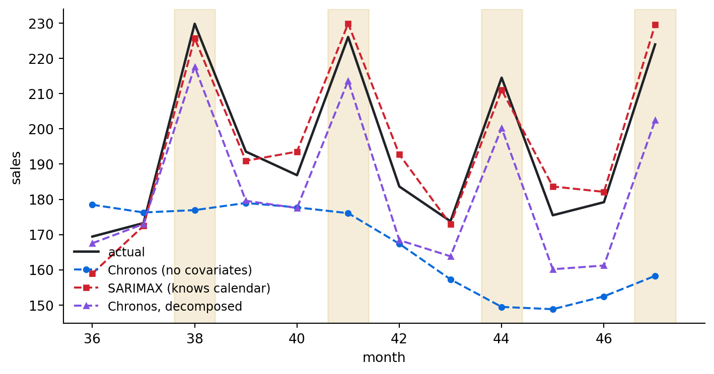
The shaded months are promotions. The covariate model rises to meet each spike because it was told the calendar; the plain foundation model forecasts the underlying rhythm and misses every spike, because the information was never in the series; a univariate forecaster with perfect pretraining would miss them too. The decomposed forecast is the interesting row: in our run it closes most of the gap to the covariate model, with the residual error tracking how well the simple uplift estimate matched the true effect. The caveats are built into its method: one additive uplift estimated from a handful of promo months is a crude model of a promotion, and with overlapping drivers, uplift that varies by season, or too few historical promos to average over, the subtraction degrades, which is when the covariate-capable models (the newer foundation models in the family paragraph above, or a classical model with exogenous inputs) are worth reaching for. The practical rule: if known drivers move your series, hand the model the calendar or decompose it out, and measure both against the held-out months. What does not work is hoping a univariate forecaster will infer a marketing calendar from sales history alone.
20.7 Choosing your multimodal stack
In Part VII we transcribed speech, read images, and forecast a series. Each of these modalities has open models you can run and hosted ones you can call.
| Capability | Open-weight | Hosted | Choose by |
|---|---|---|---|
| Speech to text | Whisper, faster-whisper, WhisperX, NeMo Parakeet | Deepgram, AssemblyAI, OpenAI | local against API, with pyannote for diarization |
| Vision-language | Qwen-VL, InternVL | GPT, Claude, Gemini | document volume and privacy |
| Forecasting | Chronos, TimesFM, Moirai | TimeGPT | running locally against an endpoint |
Important
- Hold ground truth so transcription and forecasts are measured, since a demonstration alone cannot show accuracy (Chapters 18, 20).
- A vision-language model reads printed text and labels closely; an unlabeled quantity is only an estimate (Chapter 19).
- Read the forecast’s uncertainty band, since the point line alone does not show the risk (Chapter 20).
Common failure points
- Trusting a vision model’s count of something it had to estimate by eye (Chapter 19).
- Taking a transcript as exact without checking word error rate on your own audio (Chapter 18).
- Staffing or budgeting on a forecast point and ignoring the interval (Chapter 20).
The current open-source and vendor options for these are in the tooling-landscape appendix, dated and fuller; model and provider choice is Appendix E.
20.8 Exercises
20.8.1 Conceptual questions
What does “zero-shot” mean for a time-series foundation model?
- It forecasts only a single step ahead and must be refitted for any longer horizon
- It forecasts a series it has never seen, with no training step on that series
- It produces a forecast without needing any historical context as input
- It was pretrained on the exact series it is later asked to forecast
Chronos returns a set of quantiles for each future month. Compared with a single forecast line, this gives you:
- A faster forecast, since quantiles are cheaper to compute than a full mean
- Several independent forecasts that you can average into one more accurate line
- The trend and seasonal components of the series, separated for inspection
- An uncertainty band, the range the true value should fall in most of the time
Why does the uncertainty band widen as the forecast reaches further out?
- Longer horizons leave the model fewer context points to condition each step on
- The model compounds rounding errors with every additional month it predicts
- The model is genuinely less certain about the distant future, and reports it
- The band widens by a fixed percentage per step as a plotting convention
The naive baseline in forecasting is:
- Repeating the last observed value for every month of the horizon
- Projecting the average of the entire history forward unchanged
- Drawing a straight line through the first and last points of the series
- Refitting a small ARIMA model each month as new data arrives
On the held-out year, the MAEs were Chronos 16.8, naive 18.9, and SARIMA 6.5. The chapter’s reading is:
- Chronos failed here, and foundation models are not yet ready for forecasting work
- SARIMA’s win shows pretraining adds nothing once a series has clear seasonality
- The twelve-month test window was unrepresentative, so the comparison should be rerun on more data
- The fitted model wins on its own series; the foundation model’s edge is scale without fitting
Why does the chapter measure Chronos against SARIMA as well as the naive baseline?
- A fitted classical model is the real alternative; beating only naive proves too little
- SARIMA establishes the theoretical ceiling that no zero-shot model can exceed
- Mean absolute error is only meaningful when at least two baselines are compared
- A naive forecast cannot follow a seasonal series, so judging against it alone would be unfair
You must forecast demand for ten thousand SKUs (stock-keeping units) by next week. The chapter’s comparison points you toward:
- Fitting a separate SARIMA model to every SKU, since fitted models won on the example
- The naive forecast for every SKU, since it is the only method that scales that far
- The foundation model, since it forecasts every series with no per-series fitting
- Training a new foundation model from scratch on your own ten thousand series
The cost callout says a Chronos forecast is almost free. Where does the remaining effort go?
- Covering the per-series training cost, which still grows in step with the number of series
- Evaluating which series the model serves well, with no model built for each
- Renting the GPU cluster that the model needs to forecast at production scale
- Licensing the model, which is priced per forecast once volumes reach production
20.8.2 Build lab
Forecast three different synthetic series, one with strong seasonality, one with a sharp trend, and one that is mostly noise, and compare Chronos’s MAE to the naive baseline on each. Report which kind of series the foundation model helps most on, and which it barely beats.
20.8.3 Evaluate lab
Add a commonly stronger baseline than naive: a seasonal-naive forecast that repeats the value from twelve months earlier. Measure Chronos, naive, and seasonal-naive on the held-out months. Report whether seasonal-naive is in fact stronger here, whether Chronos still wins against it, and decide which forecaster you would deploy for this series.
TipProject ideas
This part took you beyond text, into scanned images, recorded speech, and numeric time series. These two projects build on the vision and forecasting chapters.
- Read scanned documents with a vision model. Extract structured fields (vendor, date, line items, totals) from scanned invoices or receipts, then check that the totals add up. Data to try: the SROIE or CORD receipt sets, or RVL-CDIP for mixed document types.
- Forecast a portfolio of series and flag the risky ones. Run a foundation forecaster across many related series at once (stores, products, regions), produce calibrated uncertainty intervals, and flag the series most likely to breach a threshold next period. The deliverable is a ranked watchlist a manager could act on. Data to try: the M5 competition’s hierarchical retail series, public electricity or demand data, or your own multi-series history.
The transcription pipeline from Chapter 18 makes a natural third project, turning recorded calls into the structured text the rest of the book works with. Part VIII organizes what you extract into a knowledge graph.
NoteWhere we go next
This concludes Part VII, where we went beyond text and explored models for audio, images, and time. In Part IX we return to text but organize it differently: where retrieval worked over a flat pile of chunks, in Chapter 21 we extract the entities and relationships in documents to form a knowledge graph, a structured map of who relates to what.