# Everything this chapter needs is already in the gaba-core environment.
# If you are in a fresh environment, this installs the essentials:
%pip install -q openai python-dotenv pandas tenacity2 Talking to models
APIs, prompts, caching, and when to spend reasoning tokens
Chapter 1 concluded that in the generative era the analyst’s effort concentrates in framing the problem and measuring the result, and this chapter takes up that effort in code. We make our first call to a model through its API (application programming interface), the request-and-response channel through which one program asks another for work; we then wrap that call so we never write it twice, and we turn the customer-support triage problem from a thought experiment into a script that classifies real tickets. Along the way we meet the two mechanisms that decide what a system costs: prompt caching, which makes a repeated prompt cheap, and model routing, which decides when a slow, expensive reasoning model is worth the extra cost.
NoteSetup for this chapter
Run this chapter in the gaba-core environment. If you have not done this yet, see the complete setup walkthrough in Appendix A. You will need an OPENROUTER_API_KEY in a .env file (a local file that holds secrets like API keys, kept out of your code) at the book root.
OpenRouter gives us one API that reaches many model providers, and it speaks the OpenAI protocol (the request format the openai client uses). As such, we use the standard openai package throughout this chapter.
# Load the API key from the .env file at the book root, then import what we need.
from dotenv import load_dotenv
load_dotenv()  # reads OPENROUTER_API_KEY into the environment

import pandas as pd
2.1 Tools in this chapter
| Tool | Why we use it here | Alternatives | Trade-off |
|---|---|---|---|
| OpenRouter | one key reaches many providers, speaking the OpenAI protocol | a provider’s own API; a self-run gateway like LiteLLM or Portkey | one account for many models against a dependency on the router |
openai SDK |
the client the industry uses; a different base URL points it at other providers | each provider’s own SDK | one interface everywhere against provider-specific features |
Part I closes, in Chapter 4, with the fuller picture of where models run; see the tooling-landscape appendix for the current options.
2.2 Base and instruct models
Before we start using large language models (LLMs), the text-producing foundation models introduced in Chapter 1, we need to understand the distinction between a base model and an instruct model, because the model behind any API is one of these two, and for analytics work we will almost always want the second.
Pretraining produces a base model: a next-token prediction machine that has read an enormous amount of text and learned, for any run of words, what tends to come next. It is autocomplete trained on the internet: fluent, knowledgeable, and indifferent to your intent. Given “The capital of France is”, it puts most of its probability on “Paris.” Given “Write a poem about the ocean”, it writes no poem, because it predicts the text that usually follows that sentence, which might be “and submit it to our contest by March 15.”
An instruct model is that same base model after a second stage of training on (instruction, response) pairs and human preferences, the on-the-job training that turns “predict the next token” into “do what was asked.” Handed the same prompt, the instruct version writes the poem. The knowledge was already in the base model; instruction tuning taught it to apply that knowledge on request.
This difference is why model names carry a suffix: Llama-3.1-8B-Instruct. Every call in this book goes to an instruct model, because we want a system that answers, classifies, and extracts on command, whereas a base model free-associates. When a model offers both a base and an instruct (or “chat”) variant, the instruct variant is the one to call.
The mechanism of instruction tuning also predicts when a model will be reliable. Instruction tuning works from examples of recurring task families, and from them the model learns a task template for each: what a direct answer to a question looks like, how a summary condenses an article, what “translate to Spanish” should return. A request that resembles a familiar task family lands on a learned template and is handled reliably, while a genuinely novel request falls between the templates, and the model improvises by blending the nearest ones. The blend is often good enough and sometimes confidently wrong.
A map makes the idea concrete:
2.3 The first call
We reach the model through its API: our code sends a request over the network to a service running on someone else’s computer and receives a response. For language models this is the default, since the strongest models are too large to run on a laptop, and as such providers expose them only as a service. Running an open model on your own hardware is the principal alternative, which we examine in Chapter 4; for everything in this chapter, an API call is the fastest path and costs a fraction of a cent.
A language model behind an API is, from our side, a function. We send it some text and a few settings, and it returns some text. The settings matter, so let us make one call with the raw SDK (software development kit, the provider’s official client library) and examine every part of it before we conceal these details behind a wrapper.
OpenRouter exposes an OpenAI-compatible endpoint. This means we use the same openai client the whole industry uses, and only change two things: the base URL and the API key. By default, the client sends its requests to OpenAI, but with the base URL set to OpenRouter’s, it sends them to OpenRouter.
import os
import openai

# OpenRouter speaks the OpenAI protocol. We point the standard client at
# OpenRouter's URL and hand it the OpenRouter key. Nothing else changes.
client = openai.OpenAI(
    base_url="https://openrouter.ai/api/v1",
    api_key=os.environ["OPENROUTER_API_KEY"],
)

# The call itself. Three things matter here:
#   - model:       which model answers. This is a cheap, fast one.
#   - messages:    the conversation, as a list of role/content dicts.
#   - temperature: how much randomness. 0 means "give me the most likely answer".
response = client.chat.completions.create(
    model="google/gemini-3.1-flash-lite",
    messages=[
        {"role": "user", "content": "In one sentence, what is a customer support ticket?"}
    ],
    temperature=0,
)

print(response.choices[0].message.content)
A customer support ticket is a digital record used by organizations to track, manage, and resolve a specific inquiry, issue, or request submitted by a customer.The reply is stored in response.choices[0].message.content. The path is verbose because a response can contain more than one choice as well as other metadata, but in practice, we will almost always want the text of the first choice.
The response also tells us what the call cost us in tokens. Tokens are what models use to read and write information, somewhat like characters we use when writing. They are subword chunks from a fixed vocabulary that can be different for every model. Every cost, context limit, and truncation in this book is denominated in tokens. We use Hugging Face’s transformers library (its open-source toolkit for pretrained models) here only to load a tokenizer and count tokens, without running any model. Note how the tokenizer breaks up the input language into tokens:
from transformers import AutoTokenizer
from IPython.display import HTML
tk = AutoTokenizer.from_pretrained("Qwen/Qwen2.5-1.5B-Instruct")
COLORS = ["#cfe3ff", "#ffd9cc", "#d8f5d3", "#f3ddff", "#ffeec2"]
samples = [
"The quarterly report was late.",
"Cryptocurrency arbitrage notwithstanding, we proceed.",
"Refund order ORD-58213 immediately.",
]
rows = []
for text in samples:
ids = tk(text)["input_ids"]
pieces = [tk.decode([i]) for i in ids]
spans = "".join(
f'<span style="background:{COLORS[j % len(COLORS)]};color:#1f2328;'
f'padding:1px 2px;border-radius:3px;">{p.replace(" ", "␣")}</span>'
for j, p in enumerate(pieces))
rows.append(f'<div style="font-family:monospace;font-size:14px;'
f'margin:4px 0;">{spans} <span style="color:#57606a;">'
f'({len(ids)} tokens, {len(text)} chars)</span></div>')
HTML("".join(rows))The␣quarterly␣report␣was␣late. (6 tokens, 30 chars)
Cryptocurrency␣arbitrage␣notwithstanding,␣we␣proceed. (9 tokens, 53 chars)
Refund␣order␣ORD-58213␣immediately. (12 tokens, 35 chars)
Read the splits, because they explain the economics. Everyday words are single tokens; “Cryptocurrency” and “arbitrage” each split in two; and the order ID, absent from any tokenizer’s vocabulary, costs a token per fragment. Text full of codes, names, and jargon is more expensive per word than plain prose. We are billed per token, separately for what we send (input) and what we get back (output), so this is the number every cost callout in the book is built from. Tokens also govern more than the bill: a model produces its reply one token at a time, so a longer output takes proportionally longer to arrive, and on self-hosted hardware, where billing is not a concern, every token still occupies compute and memory. A task accomplished in fewer tokens is therefore cheaper, faster, and a better use of the machine, whoever owns it.
# Token accounting. Input and output are billed at different rates, so we keep
# them separate.
usage = response.usage
print(f"input tokens:  {usage.prompt_tokens}")
print(f"output tokens: {usage.completion_tokens}")
input tokens: 11
output tokens: 31Tokens also define the model’s hard limit: the context window, or the maximum number of tokens a single call can hold, prompt and reply together. Everything you send shares this one budget: the system prompt, any examples, the conversation so far, whatever documents you attach, the question itself, and the space reserved for the answer. When the budget runs out, something is dropped, and which part is dropped is a design decision, made either deliberately or by default. We manage this budget deliberately in Chapter 10; here is what it looks like filling up:
2.4 A reusable wrapper: the gaba package
We just wrote eight lines to make one call to the LLM API. If we copy those eight lines into every notebook in this book, then the day OpenRouter changes its URL, or we decide to add retries, or we want every call to report its cost, we are editing thirty notebooks. Duplicated code multiplies the cost of every later change.
So we put the call in one place: a small package named gaba that accompanies this book. It is installed once per environment (pip install -e .), and every chapter imports from it. This is the same instinct that makes you replace a repeated block of code with a function, applied one level higher.
TipWith an AI coding tool
Wrapping a verbose SDK call in a clean function is exactly the kind of thing to hand to an AI coding tool. Ask it to draft call_llm, then read every line and check it does what you would have written. The version in gaba/llm.py adds retries and cost tracking; open it and read it before you use it.
Here is the wrapper we use for the rest of the book. It does three things the raw call does not: it reads the key and builds the client for us, it retries transient network failures, and it returns the cost alongside the text. The import also pulls in the gaba model-tier constants: MODEL_LIGHT for fast cheap work, MODEL_DEFAULT for general use, and MODEL_REASONING for hard problems. Each names a real model in gaba/llm.py and can be overridden from your .env (the GABA_MODEL_* entries in .env.example), so when a model is eventually retired, one line repoints every example in the book.
# The book's shared LLM helper. Same call as above, but it also retries on
# flaky connections and hands back token counts and an estimated cost.
from gaba.llm import call_llm, MODEL_DEFAULT, MODEL_LIGHT, MODEL_REASONING

result = call_llm("In one sentence, what is a customer support ticket?")

print(result.text)
print()
print(f"model: {result.model}")
print(f"tokens in/out: {result.input_tokens}/{result.output_tokens}")
print(f"cost: ${result.cost_usd:.6f}")
A customer support ticket is a digital record used by organizations to track, manage, and resolve a specific inquiry, issue, or request submitted by a customer.
model: google/gemini-3.1-flash-lite
tokens in/out: 11/31
cost: $0.000049call_llm returns an LLMResult with the text and the bookkeeping. From here on we use it wherever we would have used the raw client, and we stop thinking about base URLs.
WarningDon’t outsource this
One short call costs a tiny fraction of a cent. That figure anchors every later cost check, because a thousand calls in a loop should cost roughly a thousand times it, and a total far from that expectation means something is wrong. Noticing is a job the tool will not do for you.
2.5 Prompts: system, user, and temperature
The messages list can contain more than one role. The two we use most frequently are system and user. The system message sets the model’s standing instructions, the role it plays, and the rules it follows. The user message is the specific request. Separating them keeps the instructions in one stable place and the varying input in another, which matters for caching later in this chapter and for readability throughout.
# The system message sets the rules once. The user message carries the input.
result = call_llm(
    prompt="The product arrived smashed to pieces and I am furious.",
    system=(
        "You are a support routing assistant. Reply with a single word describing "
        "the customer's emotion. Use lowercase."
    ),
)
print(result.text)angryThe other setting worth understanding now is temperature. It controls randomness. At temperature 0 the model returns its single most likely continuation, so the same input gives essentially the same output every time. As temperature rises, the model samples less likely words more often, which reads as variety or creativity. For analytics tasks, classifying, extracting, routing, we almost always want temperature 0, because the same input should give the same output on every run. We turn it up only when variety is the point, such as generating diverse synthetic examples in Chapter 17.
# Same creative prompt twice at temperature 1: the outputs differ.
for i in range(2):
    r = call_llm(
        "Write a four-word tagline for a coffee brand.",
        temperature=1.0,
    )
    print(f"run {i + 1}: {r.text.strip()}")
run 1: Wake up your soul.
run 2: Awaken your inner soul.Run that block again and the lines change; hold temperature at 0 and the variation disappears. That predictability is why every classification call in this book sets temperature to 0, which is also the default in call_llm.
2.6 Our first triage pass
We now have all the tools we need to convert the Chapter 1 scenario into a script. The support manager wants to have every ticket sorted into a category. We have fifteen categories and thirty sample tickets. Let us classify them.
The data comes first: the tickets are stored in a CSV file that gaba.data loads for us.
from gaba.data import load_tickets, TICKET_CATEGORIES

tickets = load_tickets()
print(f"{len(tickets)} tickets, {len(TICKET_CATEGORIES)} categories:")
print(", ".join(TICKET_CATEGORIES))
tickets.head(3)
30 tickets, 15 categories:
billing_problem, refund_request, shipping_delay, damaged_item, wrong_item, account_access, technical_issue, product_question, cancellation, subscription_change, feature_request, complaint, praise, fraud_report, other| ticket_id | text | |
|---|---|---|
| 0 | T001 | I was charged twice for my order last week. Ca... |
| 1 | T002 | This is the third time my delivery has been pu... |
| 2 | T003 | The blender arrived with a cracked jar. The bo... |
The triage itself is one prompt. We give the model the list of allowed categories in the system message and the ticket text as the user message, and we ask for just the category name.
def triage_ticket(text: str):
    """Classify one ticket; return the category and the full call result."""
    # The system message lists the legal answers and fixes the output format.
    system = (
        "You are a support ticket classifier. Read the ticket and reply with "
        "exactly one category from this list, lowercase, nothing else:\n"
        + ", ".join(TICKET_CATEGORIES)
    )
    result = call_llm(prompt=text, system=system)

    # The model usually returns a clean category, but not always. We normalize
    # and fall back to 'other' if it returns something off-list. Chapter 3
    # replaces this fragile parsing with a structured output that cannot drift.
    answer = result.text.strip().lower()
    category = answer if answer in TICKET_CATEGORIES else "other"
    return category, result


# Try it on one ticket before running the whole batch.
print(tickets.loc[0, "text"])
category, _ = triage_ticket(tickets.loc[0, "text"])
print("->", category)
I was charged twice for my order last week. Can you reverse one of the charges?
-> billing_problemThat works on one ticket. Now the batch: we classify all thirty and keep the per-call bookkeeping, the cost and the token counts, so we can total and decompose it afterward. The loop reuses triage_ticket so the prompt is never re-typed, for the same reason gaba exists: a single definition absorbs every later change. This makes thirty API calls, so it takes a moment.
records = []
for _, row in tickets.iterrows():
    category, r = triage_ticket(row["text"])
    records.append(
        {
            "ticket_id": row["ticket_id"],
            "category": category,
            "cost_usd": r.cost_usd,
            "input_tokens": r.input_tokens,
            "output_tokens": r.output_tokens,
        }
    )

results = pd.DataFrame(records)
results.head(8)| ticket_id | category | cost_usd | input_tokens | output_tokens | |
|---|---|---|---|---|---|
| 0 | T001 | billing_problem | 0.000029 | 97 | 3 |
| 1 | T002 | shipping_delay | 0.000032 | 110 | 3 |
| 2 | T003 | damaged_item | 0.000029 | 96 | 3 |
| 3 | T004 | wrong_item | 0.000029 | 98 | 3 |
| 4 | T005 | account_access | 0.000030 | 100 | 3 |
| 5 | T006 | product_question | 0.000029 | 97 | 3 |
| 6 | T007 | cancellation | 0.000027 | 97 | 2 |
| 7 | T008 | subscription_change | 0.000030 | 102 | 3 |
A quick look at how the tickets spread across categories tells us whether the classifier is behaving sensibly even before we have labels to score against.
# How many tickets landed in each category?
results["category"].value_counts()
category
billing_problem 3
damaged_item 3
wrong_item 3
product_question 3
shipping_delay 2
account_access 2
cancellation 2
subscription_change 2
feature_request 2
praise 2
fraud_report 2
refund_request 2
complaint 1
technical_issue 1
Name: count, dtype: int64The distribution resembles a real support queue: a mix of billing problems, refunds, shipping and damage issues, with a few praise and fraud reports. This distribution is an encouraging sign, although a sign of this kind falls short of a measurement. We reach the measurement at the end of the chapter, and a proper accuracy score in Chapter 3 once we have labels.
2.7 Prompt caching: paying once for a stable prefix
Look again at the batch loop. Every one of the thirty calls sent the same long system message, the full list of fifteen categories and the instructions, and only the ticket text changed. We paid input tokens for that identical preamble thirty times.
Prompt caching is the fix: when a provider supports it, the result of processing a stable prefix is cached, and later calls that share the prefix are billed for it at a steep discount. This discount reflects a real saving underneath: the cached prefix is not reprocessed, so the response also begins sooner, and on self-hosted hardware, where no bill exists, the entire benefit appears as speed and freed capacity.
The pattern is simple: put everything that stays the same at the front, and everything that varies at the end. Our triage prompt is already ordered this way, with the long instructions in the system message and the short ticket in the user message. It is ready to benefit wherever caching is available, with one caveat about prefix length that the demonstration below makes visible.
→
prefix written
to the cache,
full price
to the cache,
full price
prefix cache
processed state of
the shared prefix
processed state of
the shared prefix
→
prefix restored:
discounted, without
recomputation
discounted, without
recomputation
# Watch the cache in action. Providers only cache prefixes past a minimum
# length, so we build a realistically long system prompt: a detailed policy
# block, repeated until the prefix comfortably exceeds the threshold.
from gaba.llm import get_client, MODEL_AGENT

policy_block = (
    "You are a support ticket classifier for an online retailer. Read the "
    "ticket and assign exactly one category. Rules: a duplicate charge is "
    "billing, not refund. A refund the customer was promised but never "
    "received is refund. A package that arrived broken is damage, not "
    "shipping. A charge the customer does not recognize at all is fraud. "
    "Praise mixed with a complaint counts as a complaint. Questions about "
    "how a product works are product questions even when the customer is "
    "angry. Reply with one lowercase category and nothing else. "
)
import uuid

# Provider caches persist between runs of this notebook, so we salt the
# prefix with a fresh run marker; the first call below is then guaranteed
# to miss the cache rather than hitting one left by an earlier run.
run_marker = f"[policy revision {uuid.uuid4().hex[:8]}] "
long_system = run_marker + policy_block * 14  # ~1,300 tokens, past the cache minimum

# We demo with the agent model: its provider applies prefix caching
# automatically above the minimum and reports the hit explicitly.
for call_number in (1, 2):
    raw = get_client().chat.completions.create(
        model=MODEL_AGENT,
        messages=[
            {"role": "system", "content": long_system},
            {"role": "user", "content": "My package never arrived."},
        ],
        temperature=0,
    )
    details = getattr(raw.usage, "prompt_tokens_details", None)
    cached = getattr(details, "cached_tokens", 0) or 0
    print(f"call {call_number}: {raw.usage.prompt_tokens} prompt tokens, "
          f"{cached} of them cached")
call 1: 1442 prompt tokens, 0 of them cached
call 2: 1442 prompt tokens, 1280 of them cachedThe first call processes the whole prompt at full price and writes the prefix to the cache; the second call shares the prefix and reads most of it back at a discount. The run marker at the top of the prefix exists because provider caches persist between runs: without it, rerunning this notebook inside the cache window would report even the first call as cached, served from the previous run’s prefix. The caveat mentioned above appears in this code: providers only cache prefixes above a minimum length, around 1,024 tokens for OpenAI and Sonnet-class Claude models, though some Claude models need up to 4,096; check your provider’s caching docs before counting on it.1 A prompt shorter than that reports zero cached tokens no matter how many times you repeat it, which is exactly why our thirty-ticket loop, whose system message is only a couple of hundred tokens, never triggered the cache. Caching pays off on long, stable prefixes: detailed policy documents, long instruction blocks, few-shot example sets. Many analytics tasks require repeated processing of such long prompts with little content changing, and thus benefit heavily from caching.
Beyond the prompt-length threshold, whether you see a non-zero cached count still depends on the provider, the model, and how recently the same prefix was sent. As such, it is useful to design prompts so the stable part comes first, and a large class of repeated-prompt workloads becomes cheaper at no extra effort. We translate the savings into real money in Appendix C. For now, the point to retain is that the ordering of a prompt’s parts affects its price.
To estimate the saving at a realistic scale, we apply the same arithmetic to the 10,000-ticket quarter with a policy-block prompt like the one above. The constants are illustrative; the structure of the saving carries over to real workloads.
# Project the quarter's input bill with and without a cached prefix.
# Illustrative constants; swap in your own prompt sizes and prices. The first
# call writes the cache at full price; over ten thousand calls that rounds away.
TICKETS_PER_QUARTER = 10_000
PREFIX_TOKENS = 1_300        # the stable policy block, past the cache minimum
TICKET_TOKENS = 60           # the variable part: one short ticket
PRICE_PER_M_INPUT = 0.40     # USD per million input tokens, full price
CACHE_DISCOUNT = 0.75        # cached prefix tokens billed at 25% of full price

full = (PREFIX_TOKENS + TICKET_TOKENS) * TICKETS_PER_QUARTER / 1e6 * PRICE_PER_M_INPUT
cached = (PREFIX_TOKENS * (1 - CACHE_DISCOUNT) + TICKET_TOKENS) \
    * TICKETS_PER_QUARTER / 1e6 * PRICE_PER_M_INPUT

print(f"input bill, no caching:    ${full:.2f}")
print(f"input bill, cached prefix: ${cached:.2f}")
print(f"saved on input: {1 - cached / full:.0%}")
input bill, no caching: $5.44
input bill, cached prefix: $1.54
saved on input: 72%The quarter’s input bill is reduced by roughly 70%, and the only engineering it took was putting the stable part of the prompt first. Retain the proportion, since the dollar figure rests on illustrative constants: the discount applies only to the prefix share of the prompt, so the longer the stable prefix is relative to the variable part, the closer the whole bill moves to the discounted rate.
2.8 When to spend reasoning-model tokens
So far we have used one cheap, fast model for everything, and most analytics tasks need nothing more. Some tasks, however, require the model to work through several steps in order, and for those a reasoning model, one trained to think before it answers, can be worth its higher cost. Deciding which tasks justify it is a measurement question that intuition cannot settle, so we build a miniature test set on which the cheap model will both succeed and fail: eight refund questions from a fictional policy book, four answerable in a single careful step and four containing an ordering trap, a step that must happen in the right sequence, such as removing a non-refundable fee before prorating. Every gold answer is computed by hand, so the scoring requires no model.
# Eight fictional refund questions as (tier, question, hand-computed answer).
QUESTIONS = [
    # Single-step: careful reading, one operation.
    ("single-step", "A customer was charged 3 times for the same $19.99 order "
     "because of a billing glitch. Policy: refund every duplicate charge in "
     "full. How much do we refund?", 39.98),
    ("single-step", "A customer returns all 3 items from an order, each priced "
     "$24.50. Policy: returned items are refunded in full. How much do we "
     "refund?", 73.50),
    ("single-step", "A customer returns an opened $89.00 gadget. Policy: opened "
     "items carry a flat 15% restocking fee. How much do we refund?", 75.65),
    ("single-step", "A customer cancels a $45.00 monthly plan 18 days into a "
     "30-day month. Policy: refund the unused days, prorated daily. How much "
     "do we refund?", 18.00),
    # Ordering traps: the steps must happen in the right sequence.
    # (1200 - 200) * 155/365: remove the fee BEFORE prorating.
    ("ordering trap", "A customer on a $1,200/year plan, paid in full, cancels "
     "exactly 210 days into a 365-day year. Policy: refund the unused portion "
     "prorated daily, but a one-time $200 setup fee included in the $1,200 is "
     "non-refundable. How much do we refund?", 424.66),
    # (600 - 50) * 292/365: prorate the paid price, not the list price.
    ("ordering trap", "A customer paid $600 for an annual plan after a 25% "
     "loyalty discount off the $800 list price. They cancel 73 days into a "
     "365-day year. Policy: prorate daily on the amount actually paid, and a "
     "$50 onboarding fee included in that amount is non-refundable. How much "
     "do we refund?", 440.00),
    # 40 + 60: shipping stays because the order was only partly returned.
    ("ordering trap", "A customer returns the $40 and $60 items from a "
     "three-item order ($40, $50, $60) that also carried a $12 shipping "
     "charge. Policy: returned items are refunded in full; shipping is "
     "refunded only when the entire order is returned. How much do we "
     "refund?", 100.00),
    # 180 - 90 * (180/300): remove only this item's share of the discount.
    ("ordering trap", "A $90 promo code was applied to a $300 order of two "
     "items priced $120 and $180, allocated in proportion to item price. The "
     "customer returns the $180 item. Policy: refund the item price minus its "
     "share of the discount. How much do we refund?", 126.00),
]
Now both models answer all eight. Sixteen calls, run in parallel with ThreadPoolExecutor from Python’s standard library, which gives each call its own thread so that the reasoning model’s slow answers, which would otherwise queue one after another, overlap.
import re
import time
from concurrent.futures import ThreadPoolExecutor

def ask_and_score(model: str, tier: str, question: str, gold: float) -> dict:
    """Ask one question, score the final number, record cost and wall-clock time."""
    start = time.perf_counter()
    # Generous max_tokens: a reasoning model that runs out of room mid-think
    # returns no final number, and would be scored wrong for the wrong reason.
    r = call_llm(question + " Reply with the final dollar amount only.",
                 model=model, max_tokens=8000)
    secs = time.perf_counter() - start
    # The prompt asks for the final amount only, so we score the last number.
    numbers = re.findall(r"\d[\d,]*\.?\d*", r.text)
    final = float(numbers[-1].replace(",", "")) if numbers else float("nan")
    return {"model": "cheap" if model == MODEL_DEFAULT else "reasoning",
            "tier": tier, "correct": abs(final - gold) < 0.02,
            "cost_usd": r.cost_usd, "seconds": secs}

jobs = [(m, t, q, g)
        for m in (MODEL_DEFAULT, MODEL_REASONING) for t, q, g in QUESTIONS]
with ThreadPoolExecutor(max_workers=8) as pool:
    runs = list(pool.map(lambda job: ask_and_score(*job), jobs))

summary = (
    pd.DataFrame(runs)
    .groupby(["model", "tier"])
    .agg(accuracy=("correct", "mean"),
         mean_cost_usd=("cost_usd", "mean"),
         mean_seconds=("seconds", "mean"))
    .round({"accuracy": 2, "mean_cost_usd": 5, "mean_seconds": 1})
)
summary| accuracy | mean_cost_usd | mean_seconds | ||
|---|---|---|---|---|
| model | tier | |||
| cheap | ordering trap | 0.5 | 0.00003 | 0.7 |
| single-step | 1.0 | 0.00002 | 0.5 | |
| reasoning | ordering trap | 1.0 | 0.00877 | 127.1 |
| single-step | 1.0 | 0.00352 | 67.7 |
Read the table one tier at a time. On the single-step tier both models sit at or near full marks, and when the reasoning model does drop one, the cause is characteristic: a model trained to deliberate can overthink a simple question, and a long chain of thought gives the final number more ways to go missing, through second-guessing or through running out of output tokens. On this tier the reasoning model pays a large multiple of the cost and of the latency, in this run roughly a hundred times each, for no gain in accuracy,2 so routing single-step questions to it adds cost without adding accuracy.
The ordering-trap tier is where the two models separate: the cheap model loses questions exactly where the trap sits, prorating before removing the fee, or refunding shipping it should have held back, while the reasoning model works the steps in sequence and keeps more of them. This second tier is the work a reasoning model is for, and the table yields the routing rule directly: send each task to the model its difficulty warrants, since a single model for every task either overspends on the easy tier or fails the hard one.
This one experiment displays the structure of the routing decision, although eight questions are too few to establish it; before trusting the rule on a real workload, we would measure it across a proper test set. A reasoning model improves accuracy only on the tasks the cheap model gets wrong, while on tasks the cheap model already handles it adds cost and latency without benefit. Identifying which tasks belong to which group requires measurement, the subject of Chapter 9. The sensible default policy, refined in later chapters, is therefore to send everything to the cheap model first and to escalate to a reasoning model only where measurement shows the cheap model failing. The two possible routing errors differ in kind: over-escalation wastes money and time on tasks the cheap model already handles, while under-escalation delivers wrong answers on tasks that needed the stronger model.
One more update to the mental model: by 2026, reasoning is usually a parameter whose level we can control, whereas it was once a binary choice of model. The current generation of frontier models are hybrids that expose a reasoning-effort or thinking-budget parameter, so “cheap model versus reasoning model” increasingly means one model with the dial low versus the same model with the dial high. None of that changes the routing lesson. Whether you switch models or turn a parameter, you are deciding the same thing: when to pay for thinking.
flowchart TB
    task([incoming task]) --> decide{"multi-step arithmetic<br/>or policy reasoning?"}
    decide -- "no: most traffic" --> fast["cheap, fast model"]
    decide -- "yes: the few hard cases" --> deep["reasoning model"]
    fast --> answer([answer])
    deep --> answer
2.9 Evaluation: cost and quality of the triage pass
We built a triage system, and as promised in Chapter 1, every chapter measures what it builds. Labeled data does not exist yet, so classification accuracy must wait for Chapter 3, but we can report the thing a sponsor asks about first: cost.
Metric: cost per ticket, and total cost for the batch.
Test set: the thirty sample tickets.
Baseline: none yet. This run establishes the cost baseline that every later improvement must respect.
total_cost = results["cost_usd"].sum()
per_ticket = results["cost_usd"].mean()

print(f"tickets classified: {len(results)}")
print(f"total cost:        ${total_cost:.5f}")
print(f"cost per ticket:   ${per_ticket:.6f}")
print(f"projected cost for 10,000 tickets: ${per_ticket * 10_000:.2f}")
tickets classified: 30
total cost: $0.00087
cost per ticket: $0.000029
projected cost for 10,000 tickets: $0.29This is the kind of projection that belongs in an analytics proposal written for stakeholders, because it states the cost of the actual job at its actual scale, a full quarter of tickets classified for a trivial sum, where a capability claim or a per-million-token rate states neither. The projected figure also serves as a reference point for the rest of the book. When later chapters add reranking, retrieval, or a reasoning step, each addition moves the per-ticket cost, and an addition whose extra cost cannot be justified by the value gained should not be made.
These figures are small because the example is small: we are classifying thirty short tickets with an inexpensive model matched to the task. Enterprise budgets are of a different order. In Menlo Ventures’ late-2025 survey of roughly five hundred United States enterprises, 37 percent reported spending more than $250,000 a year on large language models, and enterprise spending on generative AI as a whole roughly tripled in a year, to an estimated $37 billion.3 At that scale, the habits this chapter practices on thirty tickets, projecting the per-unit cost and justifying each addition against it, are the same habits that keep a six-figure model budget defensible.
Where inside a call does the money go? We kept the token counts per call, so we can decompose the batch in both tokens and dollars.
import matplotlib.pyplot as plt
from gaba.llm import cost_estimate

tok_in = results["input_tokens"].sum()
tok_out = results["output_tokens"].sum()
# Price each side separately to see which one drives the bill.
usd_in = cost_estimate(MODEL_DEFAULT, tok_in, 0)
usd_out = cost_estimate(MODEL_DEFAULT, 0, tok_out)

fig, axes = plt.subplots(1, 2, figsize=(7, 3.4))
panels = [("tokens", tok_in, tok_out), ("estimated dollars", usd_in, usd_out)]
for ax, (title, v_in, v_out) in zip(axes, panels):
    ax.bar(0, v_in, width=0.5, color="#0969da", label="input")
    ax.bar(0, v_out, width=0.5, bottom=v_in, color="#cf222e", label="output")
    ax.set_xticks([])
    ax.set_xlim(-1, 1)
    ax.set_title(f"{title}, 30-ticket batch")
    ax.spines[["top", "right"]].set_visible(False)
axes[0].set_ylabel("tokens")
axes[1].set_ylabel("USD")
axes[0].legend(frameon=False)
plt.tight_layout()
plt.show()

print(f"input share: {tok_in / (tok_in + tok_out):.0%} of tokens, "
      f"{usd_in / (usd_in + usd_out):.0%} of cost")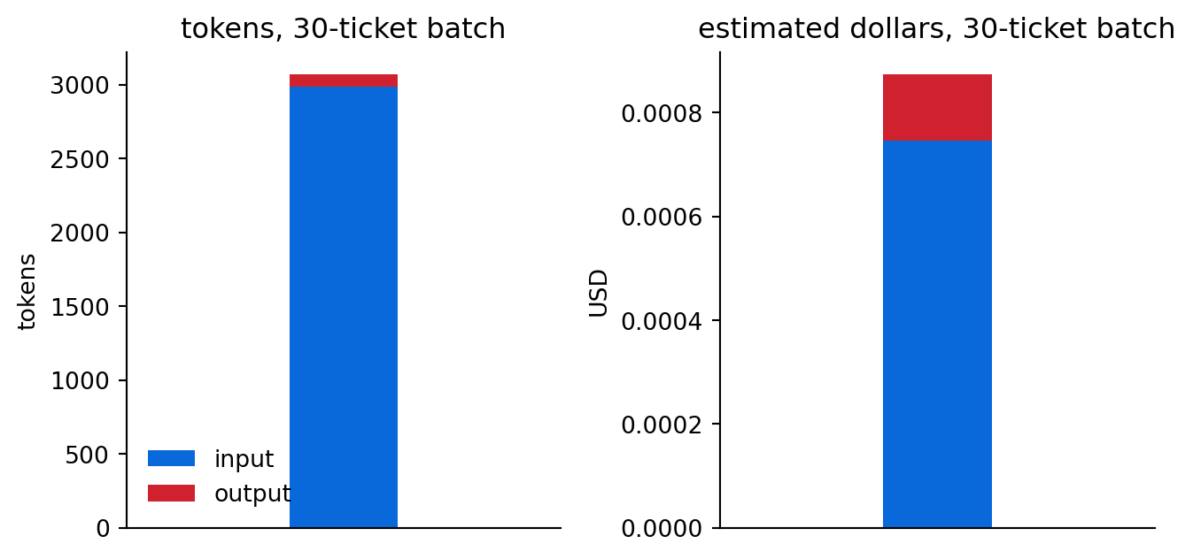
input share: 97% of tokens, 85% of costBoth panels show the same imbalance: the bill is dominated by input, since every call carries the full instruction block in and gets a single category word back. Even though output is billed at a higher per-token rate, input still dominates. This imbalance is the economic structure of classification, and it points directly back at the two input-side mechanisms this chapter taught: tighter prompts and cached prefixes affect the economics of this workload, while trimming the one-word output cannot.
TipCost: batch APIs halve the bill
Bulk work can be run more economically on batch endpoints, which the major providers offer for asynchronous jobs at typically half the per-token price, with a turnaround of up to 24 hours. Our 10,000-ticket quarterly triage is the canonical batch workload: nobody needs the categories within seconds, so an overnight batch run does the same job for about half the projected figure above. Appendix C works batch pricing into the full cost model.
On quality, our only evidence so far is the category distribution, which resembled a plausible support queue. This distributional check is qualitative; a genuine metric would require labeled tickets. As it stands, the system is cheap, fast, and unmeasured for accuracy. In Chapter 3 we constrain the output with a schema so that the format cannot drift and report the first accuracy score against the thirty labeled tickets; in Chapter 9 we assemble the full evaluation toolkit that the rest of the book applies. This is the normal sequence: the system is built first, measured next, and improved after, and until it has been measured, a system that has run is treated as unproven.
TipCost: this chapter’s example
Classifying the thirty-ticket sample cost under a thousandth of a dollar. Projected to a full quarter of ten thousand tickets, the triage runs for roughly thirty cents on the default model, the figure measured just above. Real tickets are longer than our samples, so the true figure stays well under a dollar either way. The two mechanisms from this chapter move that figure: caching cuts the repeated-prefix cost where the provider supports it, and routing keeps slow reasoning models off tasks that do not need them.
ImportantCompliance: tickets carry personal data
The tickets we just sent to a third-party API contain customer complaints, and real ones would carry names, order numbers, and email addresses. The moment we put customer data in a prompt, we are making a data-processing decision with legal weight. Appendix D has the decision flowchart for when this crosses into regulated territory and how to redact before the call. The point appears this early because the very first useful system we built already processes such data.
2.10 Exercises
2.10.1 Conceptual questions
Repointing the standard
openaiclient from OpenAI to OpenRouter requires changing which two things?- The model name and the temperature setting
- The system message and the user message
- The retry policy and the token limit
- The base URL and the API key
A classification pipeline returns different answers on identical input across runs. The most likely cause is:
- The temperature is set above zero
- The provider’s prompt cache expired between the runs
- The API key was rotated between the two runs
- The system message is longer than the user message
Why put the long, fixed instructions in the system message and the short, varying ticket in the user message?
- The OpenAI protocol requires standing instructions to be placed in the system role
- System messages are billed at a lower per-token rate than user messages
- It puts the cacheable stable prefix first and keeps instructions together
- The model weighs system messages more heavily than user messages
You are reporting the cost of the triage system to a sponsor. Which figure serves them best?
- The model’s posted price per million input and output tokens
- The projected cost of classifying a full quarter of tickets
- The average number of output tokens each classification call produces
- The model’s ranking on a public capability leaderboard
A teammate routes every ticket, including one-word classifications, through a reasoning model “to be safe”. The clearest problem is:
- It pays reasoning-model cost and latency with no gain in accuracy
- Reasoning models cannot hold temperature at zero for classification
- Reasoning models refuse to return short single-word answers
- The shared prompt prefix can no longer be cached by the provider
The routing test set includes an annual-plan question where a $1,200 payment contains a non-refundable $200 setup fee. Which failure is that ordering trap designed to catch?
- The reasoning model ran out of tokens before reaching a final figure
- Both models missed it, showing the question needed a human reviewer
- The cheap model refused to answer without more policy details
- The cheap model prorated the full $1,200 before removing the setup fee
The chapter’s evaluation section reports cost but not accuracy. Why?
- Accuracy is not a meaningful metric for a classification task
- No labeled tickets exist yet, so accuracy must wait for Chapter 3
- The cost figure already tells us how accurate the system is
- The category distribution already proves the classifier is accurate
One short call costs a tiny fraction of a cent, and the chapter asks you to remember that number. Why?
- Because per-token rates change often and the anchor needs refreshing
- Because the per-call figure is the headline number a sponsor wants to see
- So a batch total far from a thousand times it signals something is wrong
- Because it determines when self-hosting becomes cheaper than the API
2.10.2 Build lab
Extend triage_ticket so it returns both a category and a priority of low, medium, or high. A furious customer reporting fraud is high; a product question is low. You may use an AI coding tool to draft the change. Read every line you accept, and mark tool-drafted lines with a # <tool>: comment. Run it on the thirty tickets and show the priority distribution.
2.10.3 Evaluate lab
Run the full thirty-ticket batch twice: once with MODEL_DEFAULT and once with MODEL_LIGHT. For each run, record total cost, cost per ticket, and total wall-clock time. Put the six numbers in a small table. Then write two sentences: which model would you choose for this task, and what number defends the choice? You may use a tool to write the timing loop. You must choose the metric and read the result yourself.
NoteWhere we go next
Our triage parser is fragile: it trusts the model to return a clean category and falls back to “other” when it does not. Chapter 3 fixes this properly with structured outputs, so the model returns typed, validated data we can load straight into a dataframe, and the parsing step stops being a place where errors hide.
OpenAI caches prefixes above 1,024 tokens; Anthropic’s minimum ranges from 1,024 to 4,096 tokens depending on the model. See the OpenAI and Anthropic prompt-caching documentation.↩︎
On OpenRouter, the tokens a reasoning model spends thinking are billed and counted even when they never appear in the visible answer, which is why its cost runs high even on short replies.↩︎
Menlo Ventures, “2025: The State of Generative AI in the Enterprise,” December 2025, https://menlovc.com/perspective/2025-the-state-of-generative-ai-in-the-enterprise/. Verified July 2026.↩︎