import numpy as np
import pandas as pd6 Embeddings and vector search
Searching a corpus by meaning
In Chapter 5 we turned one document into clean text. A real corpus is hundreds or thousands of documents, and once reading any one of them is a solved problem, the hard question becomes how to find the few that answer a question. Keyword search is the obvious tool and it fails in a specific, frustrating way: because it matches only words, a search for “shipping delays” misses a document that says “the order still has not arrived,” even though the two mean the same thing. This is the bottom rung of the ladder from Chapter 1, where rules match exact words, a trained classifier matches patterns of wording, and a generative model responds to what the customer meant. Embeddings are where “same intent, different words” becomes a measurable distance: we turn text into vectors that capture meaning, store them in a vector database, and search a corpus of annual reports by what we mean, whatever exact words we type.
NoteIn the running system
This is the index behind our desk’s document answers. Embedding the filings here is what lets a question find the right passage by meaning, the step Chapter 7 turns into a grounded answer.
NoteSetup for this chapter
Run in the gaba-core environment. This chapter introduces gaba.embed.embed_texts, which uses the BGE-M3 model (an open-weight embedding model from BAAI). The first run downloads the model (about 2 GB) from Hugging Face into the local cache, with later runs loading from disk; embedding the small corpus here takes under a minute on a modern CPU, and the chunk-size sweep near the end re-embeds it three more times, which adds several minutes on CPU and seconds on a GPU. The corpus is eight annual reports in assets/data/filings/, .md files we produced with Chapter 5’s extractor from the companies’ 2023 annual reports: Amazon, Tesla, Bank of America, Hormel Foods, Black Hills, Ambac, Air Transport Services Group, and Park Hotels.
6.1 Tools in this chapter
| Tool | Why we use it here | Alternatives | Trade-off |
|---|---|---|---|
| BGE-M3 (embeddings) | open-weight, runs locally with no per-call fee, and returns a sparse vector alongside the dense one (Chapter 8 uses the sparse half) | OpenAI text-embedding-3, Cohere, Voyage (hosted) | local control against an API you do not operate |
| ChromaDB (vector store) | in-process, needs no server, and handles far more than this corpus | Qdrant or Milvus (self-hosted), Pinecone (managed), pgvector | simplicity now against scale later |
Part II closes, in Chapter 7, with the document stack as a whole. The current options are listed in the tooling-landscape appendix.
6.2 What an embedding is
An embedding turns a piece of text into a list of numbers, a vector, positioned so that texts with similar meaning sit near each other. “Near” has a precise definition: the cosine similarity between two vectors, which is 1 when they point the same way and 0 when they are orthogonal. Because BGE-M3 returns normalized vectors (each scaled to unit length), that similarity is just their dot product. One thing to expect: real text embeddings are not spread out to fill the space, so even unrelated sentences usually score well above 0. Read a similarity matrix by comparing values to each other, because the absolute zero is a reference no real pair of texts approaches.
The most convincing demonstration is to examine it directly. Here are six short sentences on three topics: growth, an executive leaving, and cost pressure. Within each pair, the two sentences mean roughly the same thing while sharing almost no words.
from gaba.embed import embed_texts

sentences = [
    "Revenue increased sharply this quarter.",          # growth
    "Sales grew strongly compared to last year.",       # growth, different words
    "The chief executive announced her resignation.",   # departure
    "Our top leader is stepping down from the role.",   # departure, different words
    "Raw material costs squeezed our margins.",         # costs
    "Higher input prices cut into profitability.",      # costs, different words
]
labels = ["growth-1", "growth-2", "depart-1", "depart-2", "cost-1", "cost-2"]

vectors = embed_texts(sentences)  # shape (6, 1024)

# Cosine similarity is the dot product for these normalized vectors.
sim = vectors @ vectors.T
pd.DataFrame(np.round(sim, 2), index=labels, columns=labels)| growth-1 | growth-2 | depart-1 | depart-2 | cost-1 | cost-2 | |
|---|---|---|---|---|---|---|
| growth-1 | 1.00 | 0.81 | 0.52 | 0.47 | 0.61 | 0.65 |
| growth-2 | 0.81 | 1.00 | 0.49 | 0.50 | 0.57 | 0.60 |
| depart-1 | 0.52 | 0.49 | 1.00 | 0.77 | 0.49 | 0.55 |
| depart-2 | 0.47 | 0.50 | 0.77 | 1.00 | 0.51 | 0.55 |
| cost-1 | 0.61 | 0.57 | 0.49 | 0.51 | 1.00 | 0.78 |
| cost-2 | 0.65 | 0.60 | 0.55 | 0.55 | 0.78 | 1.00 |
Read the matrix: each sentence is most similar to its topic partner, even though the pairs share almost no words, and similarity drops across topics. The model has grouped the sentences by meaning, and this grouping is the entire idea; everything else in this chapter is plumbing around it.
The same numbers read faster as a heatmap, where the structure appears before any individual value does: three bright blocks along the diagonal, one per topic pair, on a dimmer background of cross-topic scores.
import matplotlib.pyplot as plt

fig, ax = plt.subplots(figsize=(6, 4.8))
im = ax.imshow(sim, cmap="Blues", vmin=0.3, vmax=1.0)
ax.set_xticks(range(len(labels)), labels, rotation=45, ha="right")
ax.set_yticks(range(len(labels)), labels)
for i in range(len(labels)):
    for j in range(len(labels)):
        ax.text(j, i, f"{sim[i, j]:.2f}", ha="center", va="center", fontsize=8,
                color="white" if sim[i, j] > 0.8 else "#1f2328")
fig.colorbar(im, ax=ax, shrink=0.85, label="cosine similarity")
plt.tight_layout()
plt.show()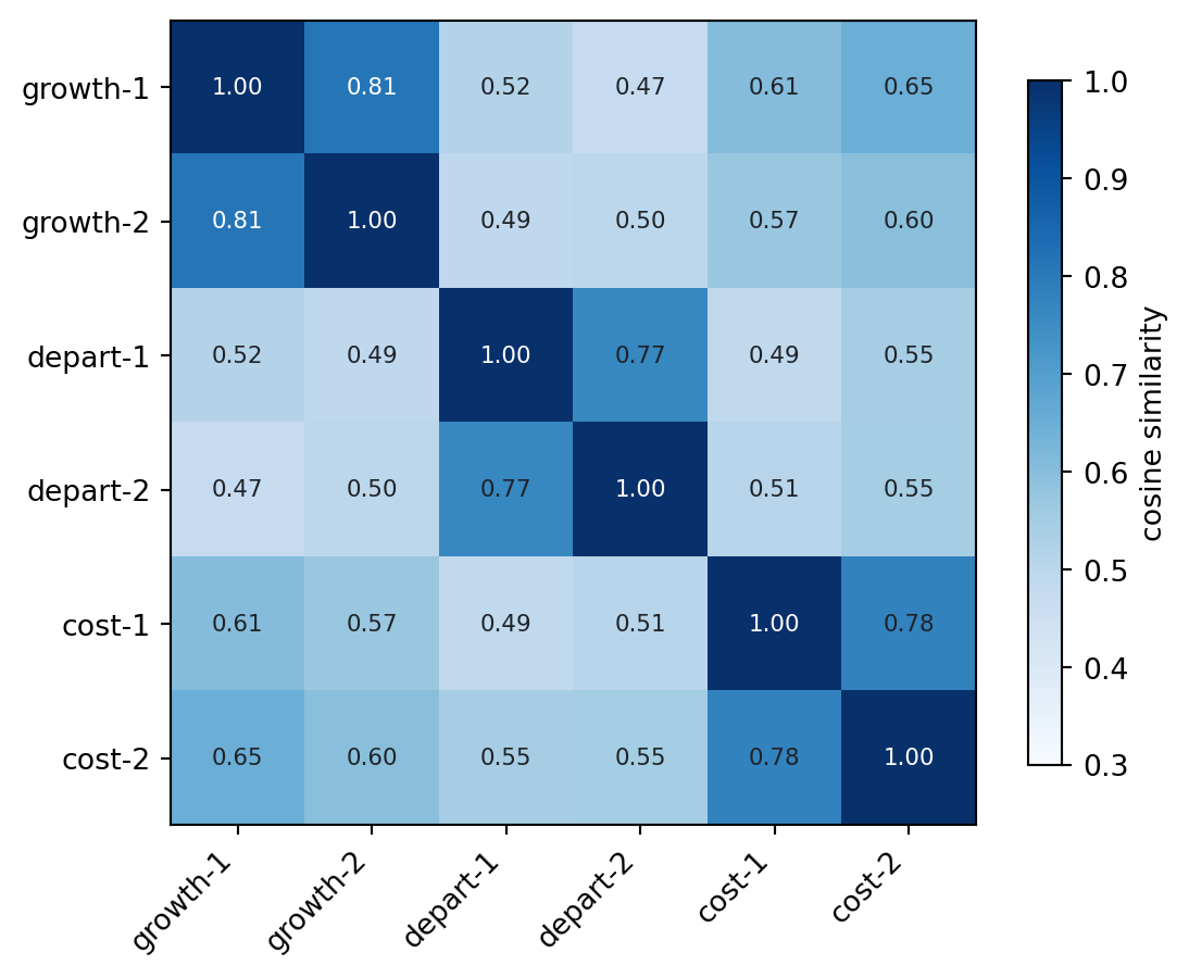
A map makes the same point one more way. The vectors have 1,024 dimensions, which we cannot draw, but principal component analysis (PCA) can project them onto the two directions along which they differ most. In the projection each pair stays together and the topics stay apart.
from sklearn.decomposition import PCA
import plotly.express as px

coords = PCA(n_components=2, random_state=0).fit_transform(vectors)
topics = [label.split("-")[0] for label in labels]

fig = px.scatter(
    x=coords[:, 0], y=coords[:, 1], color=topics, text=labels,
    hover_name=sentences,
    color_discrete_map={"growth": "#0969da", "depart": "#cf222e", "cost": "#8250df"},
    labels={"x": "first principal component", "y": "second principal component", "color": "topic"},
)
fig.update_traces(
    marker=dict(size=14, opacity=0.85), textposition="top center",
    hovertemplate="%{hovertext}<extra>%{fullData.name}</extra>",
)
fig.update_layout(height=440, margin=dict(l=10, r=10, t=20, b=10))
fig.show()The projection throws away most of the 1,024 dimensions, so distances on the page are a simplification of distances in the full space. However, the grouping it shows is real: it is the same structure the similarity matrix reported, now in drawn form.
6.3 The limits of keyword search
Keyword search would treat “revenue increased” and “sales grew” as unrelated, because they share no words. For a support inbox or a document corpus, that is a real failure: the relevant text rarely uses the exact words of the query. Embeddings close that gap by matching on meaning, which is why we build every retrieval system in the rest of this book on them. (Keyword matching still has value, and Chapter 8 brings it back as one half of a hybrid; on its own it is not enough.) We measure that claim: once this chapter has an evaluation harness, we run keyword search and embedding search on the same queries.
flowchart LR
    q["Query:<br/>'shipping delays'"]
    a["Document A:<br/>'Shipping delays affected<br/>our fulfillment centers.'"]
    b["Document B:<br/>'The order still<br/>has not arrived.'"]
    q -- "keyword: match<br/>embedding: match" --> a
    q -- "keyword: no shared words, missed<br/>embedding: match" --> b
6.4 Building a searchable corpus
To search real documents we do three things: split each document into chunks small enough to be specific, embed every chunk, and store the vectors in a database built for similarity search. We chunk because a whole annual report is too coarse; if we embed the entire document as one vector, a query about cash flow and a query about executive pay both match the same blob. Smaller chunks give sharper matches.
WarningDon’t outsource this
An assistant can write a chunker in seconds, and you should let it. It cannot choose your chunk size for you. Too large and a query matches a vague blob; too small and a chunk loses the context that gives it meaning. That number is a judgment about your documents and your queries, and the only way to set it is to measure retrieval at a few sizes, which is yours to do.
import re
from gaba import DATA_DIR
def chunk_markdown(text: str, size: int = 900, cap: int = 70) -> list[str]:
"""Group paragraphs into chunks of roughly `size` characters."""
paragraphs = [p.strip() for p in re.split(r"\n\s*\n", text) if len(p.strip()) > 40]
# Drop extraction artifacts: image placeholders and separator runs of
# dashes/braces that carry no prose worth embedding.
paragraphs = [p for p in paragraphs if " for c in p) > len(p) * 0.5]
chunks, buffer = [], ""
for para in paragraphs:
if len(buffer) + len(para) < size:
buffer += " " + para
else:
if buffer:
chunks.append(buffer.strip())
buffer = para
if buffer:
chunks.append(buffer.strip())
return chunks[:cap] # cap per document; raise it for a larger corpus
# Eight annual reports, one per company, tagged by ticker. The same map
# is defined in gaba.rag.REPORTS, which later chapters import.
reports = {
"AMBC": "NASDAQ_AMBC_2023.md", "AMZN": "NASDAQ_AMZN_2023.md",
"ATSG": "NASDAQ_ATSG_2023.md", "BAC": "NYSE_BAC_2023.md",
"BKH": "NYSE_BKH_2023.md", "HRL": "NYSE_HRL_2023.md",
"PK": "NYSE_PK_2023.md", "TSLA": "NASDAQ_TSLA_2023.md",
}
documents, tickers = [], []
for ticker, filename in reports.items():
text = (DATA_DIR / "filings" / filename).read_text()
for c in chunk_markdown(text):
documents.append(c)
tickers.append(ticker)
print(f"{len(documents)} chunks across {len(reports)} companies")560 chunks across 8 companiesThe cap matters here: at 70 chunks per document we are indexing only the front portion of each long report, a deliberate trade to keep the chapter’s embedding step fast. The build lab raises the cap to cover full documents.
Now embed every chunk. This is the slow step, a single pass of the model over a few hundred chunks.
chunk_vectors = embed_texts(documents)
print("embedded:", chunk_vectors.shape)
embedded: (560, 1024)And store them in ChromaDB, a vector database that indexes the vectors so we can ask for nearest neighbors quickly. We tell it to measure distance by cosine similarity, since that is how the model was trained.
TipWith an AI coding tool
The create_collection and add calls below are the type of plumbing an assistant writes well: the arguments are correct and there are no surprises. Read the draft anyway, and pay attention to the metadata you are instructed to attach to each chunk. The ticker field stored here is what Chapter 7’s filtering depends on later, so the field you allow the assistant to name and fill now is the one you will need to query on then.
import chromadb

client = chromadb.Client()  # in-memory for the chapter
collection = client.create_collection(
    "reports", metadata={"hnsw:space": "cosine"}
)
collection.add(
    ids=[str(i) for i in range(len(documents))],
    embeddings=chunk_vectors.tolist(),
    documents=documents,
    metadatas=[{"ticker": t} for t in tickers],
)
print("collection size:", collection.count())
collection size: 560One calibration is in order before we search. The opening of this chapter warned that real text embeddings do not spread out to fill the space, and indeed even unrelated texts score well above zero. With a few hundred embedded chunks in hand, we can measure that floor directly by drawing random pairs of chunks, mostly unrelated passages from different companies’ reports, and computing their cosine similarities.
rng = np.random.default_rng(0)
pair_idx = rng.integers(0, len(chunk_vectors), size=(2000, 2))
pair_idx = pair_idx[pair_idx[:, 0] != pair_idx[:, 1]]
pair_sims = np.einsum(
    "ij,ij->i", chunk_vectors[pair_idx[:, 0]], chunk_vectors[pair_idx[:, 1]]
)

# The two reference scores from the sentence demo at the top of the chapter.
topic_of = [lab.split("-")[0] for lab in labels]
upper = [(i, j) for i in range(len(labels)) for j in range(i + 1, len(labels))]
same_topic = np.mean([sim[i, j] for i, j in upper if topic_of[i] == topic_of[j]])
cross_topic = np.mean([sim[i, j] for i, j in upper if topic_of[i] != topic_of[j]])

fig, ax = plt.subplots(figsize=(6.5, 4))
ax.hist(pair_sims, bins=40, color="#9a9a9a", edgecolor="white")
ax.axvline(cross_topic, color="#cf222e", linestyle="--", linewidth=1.5)
ax.axvline(same_topic, color="#0969da", linestyle="--", linewidth=1.5)
top = ax.get_ylim()[1]
ax.text(cross_topic, top * 0.96, " cross-topic\n sentences", color="#cf222e",
        fontsize=9, va="top")
ax.text(same_topic, top * 0.96, " same-topic\n sentences", color="#0969da",
        fontsize=9, va="top")
ax.set_xlabel("cosine similarity of a random chunk pair")
ax.set_ylabel("count")
ax.spines[["top", "right"]].set_visible(False)
plt.tight_layout()
plt.show()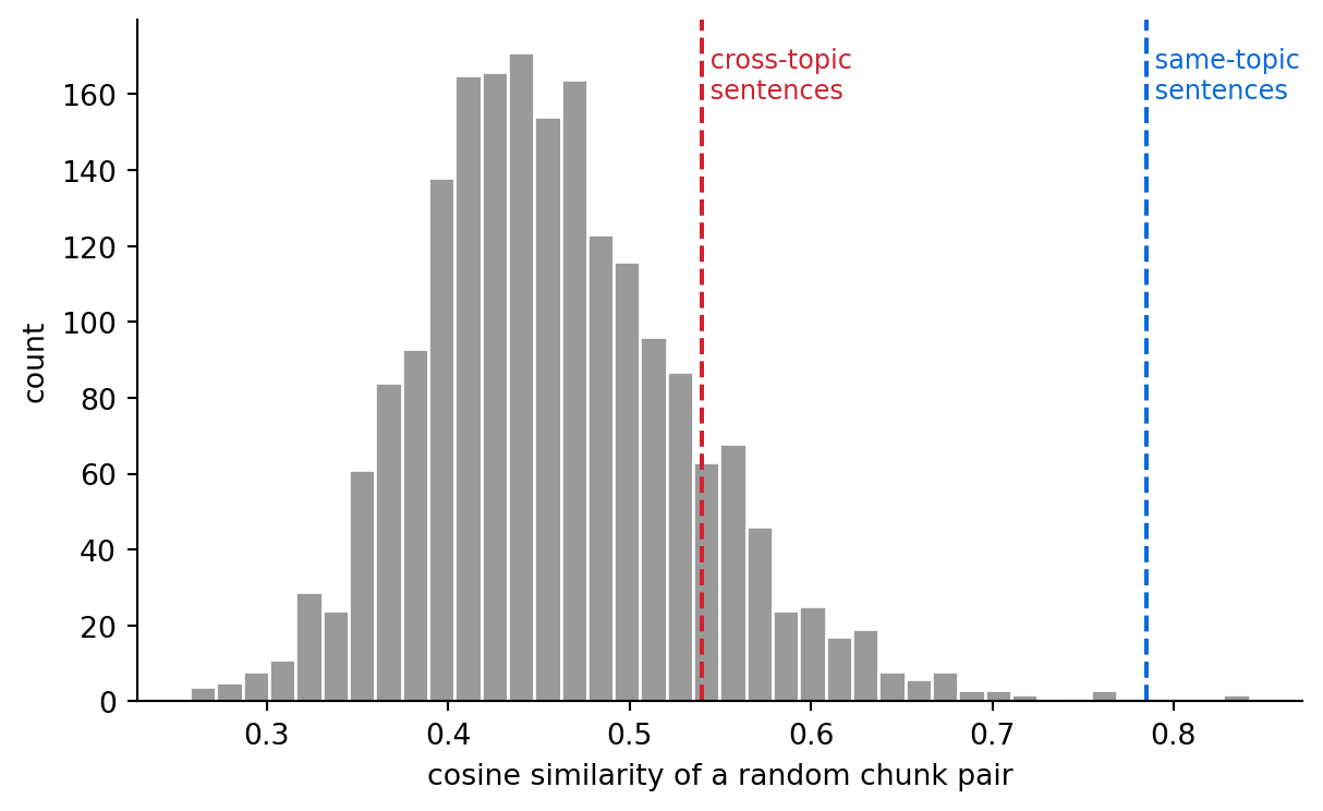
This histogram is the calibration the opening promised. Unrelated chunks in this space score roughly 0.35 to 0.6, a range that contains the cross-topic sentence scores from the demo, which therefore sat at the floor of the space and indicated no genuine similarity. The same-topic score stands outside the entire unrelated distribution, and a retrieval system depends on this separation, since the absolute value of a score carries no meaning on its own. Whenever you read a similarity score in this book, read it against this floor.
6.5 Searching by meaning
To search, we embed the query the same way we embedded the chunks, and then ask the database for the nearest ones. Here is a question phrased in words that do not appear verbatim in any report.
def search(query: str, n: int = 3) -> pd.DataFrame:
    """Embed a query and return the n nearest chunks with their company."""
    query_vector = embed_texts([query])[0]
    result = collection.query(query_embeddings=[query_vector.tolist()], n_results=n)
    return pd.DataFrame(
        {
            "ticker": [m["ticker"] for m in result["metadatas"][0]],
            "chunk": [d[:120] + "..." for d in result["documents"][0]],
        }
    )

search("How many vehicles did the company deliver to customers?")| ticker | chunk | |
|---|---|---|
| 0 | TSLA | We currently manufacture five different consum... |
| 1 | ATSG | Our commitment to innovation and growth remain... |
| 2 | ATSG | We are a leading provider of aircraft leasing ... |
The top results come from Tesla’s report, even though we never typed “Tesla”. The query matched on meaning: vehicle deliveries are a Tesla topic, and the model knows it from the content of the chunks, without any shared keyword. This match on meaning is semantic search, the engine under every retrieval system we build from here on.
6.6 Evaluating retrieval quality
We built a search system; we now need to confirm that it retrieves relevant material. The way to find out is to ask questions whose answers we know appear in a particular document, and check whether search returns that document.
Metric: hit rate at 1, the fraction of queries whose top result comes from the correct company.
Test set: four questions, each clearly about one of the companies.
Baseline: random guessing across the eight companies would be right one time in eight; to avoid a hardcoded number, we compute it from the corpus below.
test_queries = {
    "How many vehicles were delivered?": "TSLA",
    "What were the AWS cloud segment results?": "AMZN",
    "Tell me about turkey and packaged meat products.": "HRL",
    "What were the electric and gas utility operations?": "BKH",
}

hits = 0
rows = []
for query, expected in test_queries.items():
    top_ticker = search(query, n=1)["ticker"].iloc[0]
    correct = top_ticker == expected
    hits += correct
    rows.append({"query": query[:40], "expected": expected, "got": top_ticker, "hit": correct})

pd.DataFrame(rows)| query | expected | got | hit | |
|---|---|---|---|---|
| 0 | How many vehicles were delivered? | TSLA | TSLA | True |
| 1 | What were the AWS cloud segment results? | AMZN | AMZN | True |
| 2 | Tell me about turkey and packaged meat p | HRL | HRL | True |
| 3 | What were the electric and gas utility o | BKH | BKH | True |
hit_rate = hits / len(test_queries)
random_baseline = 1 / len(reports)  # one right answer among eight companies
print(f"hit rate @ 1: {hit_rate:.0%}  (random baseline: {random_baseline:.1%})")
hit rate @ 1: 100% (random baseline: 12.5%)Search returns the right document for every query, far above the random baseline. This is a small, clean retrieval evaluation, and it is the seed of a real one. In Chapter 9, we make it rigorous with more queries, relevance judged at several ranks, and metrics like precision at k that tell us how high the right document ranked as well as whether it appeared. For now, even four queries are enough to demonstrate that the search performs as intended.
6.6.1 Keyword search, measured
The harness also lets us test the claim this chapter opened with. We claimed keyword search fails when the query and the document share no vocabulary; having so far only asserted this claim, we can now measure it. The keyword baseline is TF-IDF (term frequency-inverse document frequency), the standard bag-of-words retriever (it matches on word overlap and ignores word order), fitted over the same chunks. We give both retrievers the same eight queries: the four originals, whose wording leans on the reports’ own vocabulary, plus four paraphrases written to share as little vocabulary with the reports as we could manage, the gold company (the company each query is really about, our ground truth) unchanged.
from sklearn.feature_extraction.text import TfidfVectorizer

vectorizer = TfidfVectorizer()
doc_tfidf = vectorizer.fit_transform(documents)  # the same chunks we embedded above

def keyword_top1(query: str) -> str:
    scores = (doc_tfidf @ vectorizer.transform([query]).T).toarray().ravel()
    return tickers[int(scores.argmax())]

def embedding_top1(query: str) -> str:
    return search(query, n=1)["ticker"].iloc[0]

paraphrase_queries = {
    "How many cars did they hand over to buyers?": "TSLA",
    "How is the business of renting out computing power to other firms going?": "AMZN",
    "What does the maker of canned lunch staples sell?": "HRL",
    "Who keeps the lights on and the heat running for homes?": "BKH",
}

rows = []
for set_name, queries in [("original", test_queries),
                          ("paraphrase", paraphrase_queries)]:
    for retriever_name, top1 in [("keyword (TF-IDF)", keyword_top1),
                                 ("embedding", embedding_top1)]:
        n_hits = sum(top1(q) == expected for q, expected in queries.items())
        rows.append({"queries": set_name, "retriever": retriever_name,
                     "hit rate @ 1": n_hits / len(queries)})

pd.DataFrame(rows).pivot(index="retriever", columns="queries",
values="hit rate @ 1")| queries | original | paraphrase |
|---|---|---|
| retriever | ||
| embedding | 1.00 | 0.75 |
| keyword (TF-IDF) | 0.75 | 0.25 |
Read the table one column at a time. On the original queries, keyword search holds up respectably, because the queries borrow the reports’ own words: “vehicles,” “turkey,” “utility.” Even there it drops the AWS (Amazon Web Services) question, whose remaining words (“cloud,” “segment,” “results”) are scattered across every report. On the paraphrases the gap opens wide. TF-IDF has almost nothing to match when the query says cars handed over to buyers and the document says vehicle deliveries, and its hit rate collapses toward the random floor, while the embedding retriever keeps finding the right company. It misses once too, on the most oblique paraphrase, the one about keeping the lights on, a reminder that matching on meaning stretches much further than matching on words, but not infinitely far.
6.6.2 How chunk size moves the numbers
The chunking callout earlier said the only way to choose a chunk size is to measure retrieval at a few sizes, and we now have everything needed to do exactly that. We rebuild the corpus at three chunk sizes, small, our default, and large, keeping the 70-chunk cap fixed, re-embed each version, and score hit rate at 1 on all eight queries.
import time

all_queries = {**test_queries, **paraphrase_queries}
query_vectors = embed_texts(list(all_queries))

sweep_rows = []
for size in [300, 900, 1800]:
    docs_s, ticks_s = [], []
    for ticker, filename in reports.items():
        text = (DATA_DIR / "filings" / filename).read_text()
        for c in chunk_markdown(text, size=size):
            docs_s.append(c)
            ticks_s.append(ticker)
    start = time.perf_counter()
    vecs_s = embed_texts(docs_s)
    embed_seconds = time.perf_counter() - start
    n_hits = sum(
        ticks_s[int(np.argmax(vecs_s @ qv))] == expected
        for (q, expected), qv in zip(all_queries.items(), query_vectors)
    )
    sweep_rows.append({
        "chunk size (chars)": size,
        "chunks": len(docs_s),
        "chars indexed": sum(len(c) for c in docs_s),
        "embed seconds": round(embed_seconds, 1),
        "hit rate @ 1": round(n_hits / len(all_queries), 2),
    })

pd.DataFrame(sweep_rows)| chunk size (chars) | chunks | chars indexed | embed seconds | hit rate @ 1 | |
|---|---|---|---|---|---|
| 0 | 300 | 560 | 227785 | 57.1 | 0.88 |
| 1 | 900 | 560 | 432762 | 94.9 | 0.88 |
| 2 | 1800 | 560 | 837447 | 171.6 | 0.75 |
The reading is one sentence per column. The chunk count never moves because the cap binds at every size; what changes is how much text each chunk carries, so the characters indexed and the embedding time climb with size; and the hit rate is the verdict: the large chunks do worst in our run despite indexing the most text, because an 1,800-character chunk blends several topics into one blurry vector, exactly the failure the callout warned about. For this corpus and these queries the default size holds up, and the measurement to defend it took a dozen lines.
6.7 The limits of semantic search
The perfect score on the original four queries was easy for a reason: each query named something only one company does, vehicle deliveries, an AWS segment, so search had an unambiguous target. Generic queries behave differently. Every annual report discusses risks, financial performance, and dividends, so a query about those names no single right document.
for query in ["What were the main risks to the business?",
              "How did the company perform financially this year?",
              "What dividends were paid to shareholders?"]:
    print(f"{query[:42]:42} -> {search(query, n=3)['ticker'].tolist()}")
What were the main risks to the business? -> ['HRL', 'TSLA', 'HRL']
How did the company perform financially th -> ['HRL', 'PK', 'BKH']
What dividends were paid to shareholders? -> ['HRL', 'PK', 'BKH']The results cluster on whichever company happened to phrase the topic most like the query, because the query never asked for any company in particular. The embeddings are working as designed here, because semantic search answers the query you typed, by meaning, and nothing more. When you need a specific document, the fix is to ask specifically, name the company, or to filter the search by the metadata you stored, the ticker on each chunk, so retrieval only ranks chunks from the company you mean. Retrieval and filtering working together is a theme we return to in Chapter 10.
TipCost: embeddings are cheap, and mostly free
Embedding here is local computation on a model we downloaded once, so the marginal cost of embedding a chunk is electricity, with no API bill involved. Hosted embedding APIs exist and charge per token, but they are inexpensive, and the one-time cost of embedding a corpus is paid once and reused for every future search. On owned hardware the same arithmetic appears as time and capacity: embedding is the slow step of an index build, so the throughput of the embedding model sets how often the corpus can be re-indexed. The ongoing cost of a search system is dominated by the language model that reads the results, which we add in Chapter 7; the embeddings themselves are a minor part of it.
6.8 Exercises
6.8.1 Conceptual questions
Two sentences share no words but mean roughly the same thing. What does an embedding model do with them?
- Flags one of them as a near-duplicate and drops it from the corpus
- Lowercases both and compares them character by character
- Places their vectors close together, because it encodes meaning
- Treats them as unrelated, exactly as a keyword search would
Why do we split documents into chunks before embedding, when we could embed each whole document as one vector?
- So a query matches a specific passage, whereas a whole-document vector blurs every topic into one average
- Because the vector database rejects any document longer than a fixed limit
- Because chunking strips out boilerplate that would otherwise confuse the model
- Because embedding many small pieces costs less than embedding one large document
BGE-M3 returns normalized vectors. For these, the cosine similarity between two embeddings is simply:
- The number of words their source texts share
- The Euclidean distance between the two vectors
- The edit distance between the two source texts
- The dot product of the two vectors
A search for “How many vehicles did the company deliver?” returns Tesla chunks even though the query never says Tesla. What explains this?
- ChromaDB keeps a keyword index that links “vehicles” to the ticker TSLA
- The query embedding landed nearest the chunks about vehicle deliveries, a match on meaning
- Tesla’s report was added to the collection first, so its chunks rank higher
- A metadata filter restricted the search to the automotive company
Hit rate at 1 comes out to 100 percent on the four test queries. What is the right conclusion?
- Encouraging, but four queries is a tiny test set; a real evaluation needs more
- The system is fully validated and needs no further measurement before deployment
- The metric must be wrong, because no retrieval system reaches 100 percent
- Keyword search would necessarily have scored just as well on these queries
A generic query like “What were the main risks to the business?” returns chunks scattered across companies. What is going on?
- The embedding model is too weak for financial language and should be replaced with a larger one
- The chunks were cut too small to preserve the risk-factor sections of each report
- The vector index returns arbitrary results whenever similarity scores are tied
- Every report discusses risks, so the query names no single correct document to find
The PCA scatter plot shows the six sentence embeddings in two dimensions. What should you keep in mind when reading it?
- The distances on the page are exactly the ones the search system ranks by
- It discards most of the 1,024 dimensions, so distances on the page are approximate
- PCA reverses similarity, so the points drawn closest together are the least alike
- Each axis corresponds directly to one of the three topics in the sentences
Once the corpus is embedded, where does the ongoing cost of a search system mostly come from?
- Re-embedding the entire corpus before every new query
- The vector database, which charges for each nearest-neighbor lookup
- The language model that later reads the retrieved results
- Embedding each query through a metered hosted API
6.8.2 Build lab
Add a fifth company’s report to the corpus (an annual report you download; run it through Chapter 5’s extractor first), re-embed, and write a query that should retrieve it. Confirm it does. Note how long embedding the larger corpus takes, then raise the per-document chunk cap so each report is indexed in full, and note what that does to the chunk count and the embedding time.
6.8.3 Evaluate lab
Write five new test queries, each with a company you expect to be the right answer, and measure hit rate at 1 and at 3. Then write one harder query that is genuinely ambiguous between two companies, and report what search does with it. Decide whether that case should count as a hit, and defend your choice.
NoteWhere we go next
Search finds the right chunks, although what a user wants is an answer composed from them. Chapter 7 closes the loop: we take the chunks search returns, supply them to a language model as context, and have it compose a grounded answer that cites where it came from. This grounded, cited answer is retrieval-augmented generation, the first complete application in this book.